Barry V. Kissane
The University of Western Australia
(This study arises from my Master's dissertation at the University of Western Australia. I am grateful to Dr David Andrich for his expert supervision and for his substantial help with this article.)
INTRODUCTION
To the relatively uninitiated in mental test theory, the specific problems in measuring change or gain must be surprising. But perhaps more surprising is that, although extremely competent psychometricians and researchers have been able to identify and articulate the problems, they have not been able really to show how to overcome many of them satisfactorily.
Perhaps new approaches in the measurement of change need to be explored in order to progress substantially beyond the current state of the art in which some see that measurement of change is best avoided where possible (Cronbach & Furby, 1970). This article attempts to do this by considering more closely what may be the main aims in the study of change, and by arguing that the concern is not primarily with change as such, but with the rate of change. From this perspective, a direction of study somewhat different from the traditional follows and is briefly explored. Particular reference is made to the comparison of two intact groups of people who are receiving different treatments, and who may have different initial average status.
LINEARIZATION OF TEST SCORES
Throughout the article the discussion is focussed on the case of a single variable of ability or attitude, usually referred to generically as an ability variable. It is assumed this variable can be operationalized on a unidimensional continuum by a test composed of dichotomously scored items.
One of the main problems in the study of change using test scores is the lack of an interval level of measurement when test scores are used. This implies that equal numerical changes in test scores do not represent equal affective or cognitive changes in latent ability at different levels of the continuum. The inequality of such changes is particularly evident when floor and ceiling effects manifest themselves in pre- and post-testing. The disadvantages of these effects, and one way of overcoming them, are lucidly described by Fischer (1976).
The basic method for overcoming problems of unequal measurement intervals is to use those models of latent trait theory which characterize the qualitative responses of persons to test items in terms of person and item parameters. The simplest and most convincing model for these purposes is Rasch's simple logistic model (SLM), which has only one ability parameter for each person, and only one difficulty parameter for each item. The particular advantage of the SLM over other latent trait models is that no distributional assumptions about either person or item parameters need be made (Rasch, 1960). In addition, by being able to choose different subsets of items which conform to the model, different tests of varying difficulties can be linked in order to provide much wider tests, thus overcoming any floor and ceiling effects (Wright, 1977).
One way of taking advantage of the SLM is to construct tests according to the principles described in the book Best Test Design (Wright and Stone, 1980) and then to apply standard repeated measures analysis of variance techniques to the resulting parameter estimates. Alternatively, Fischer (1973, 1976) prefers to elaborate the SLM to the linear logistic test model (LLTM) in which the estimates of various parameters and their changes over time are made simultaneously. This approach is very efficient, and by using estimation procedures in which initial abilities are conditioned out, it becomes clear that no assumptions need be made about the specific values, or the distribution of the initial abilities.
This important conditioning feature in measurement is characteristic of all Rasch's measurement models. The elimination, however, of the initial abilities is not an innovation for the measurement of change when one has interval level of measurement. This is because, in the construction of change scores, the initial abilities are eliminated by subtraction. This can be shown as follows:
Suppose that person v has ability βv1 at time t1 and βv2 = βv1 + Δβ at time t2 = t1 + Δt. If εv1 and εv2 are the respective errors of measurement on the two occasions, then
|
βv1 (hat) = βv1 +
εv1 [where (hat) = estimated] and βv2 (hat) = βv2 + εv2 = βv1 + Δβ + εv2. |
Then the estimated change may be written as,
| βv2 (hat) - βv1 (hat) = Δβ + εv2 - εv1. |
demonstrating that the change is not directly related to the initial ability βv1. Hence distributional assumptions need be made only about the population of changes, Δβ, and not about the population of initial abilities, β1. Most traditional discussions of ANOVA, therefore, contain superfluous assumptions as they tend to ignore this elimination of initial abilities.
COMPARISONS OF CHANGE SCORES
In the following sections it will be assumed that persons can be characterized by parameters estimated from responses to appropriate selections of items which conform with, and are calibrated according to, the SLM.
The study of change is usually set in a context where the aim is to understand the various causes of change, and particularly in education, to understand the effects of various planned curricula. The most compelling evidence regarding any such effects is obtained with an experimental design in which at least one group, the treatment group say, has received some particular or special curriculum, and another group, the control group, has not. Of course, such a simple experiment is not necessarily the most efficient, but because it is the easiest framework within which to discuss various issues for illustrative purposes, it will be the one considered.
A recurrent problem in the measurement of change is that change scores are exceptionally unreliable. The unreliability is primarily manifested with respect to individual scores; if one is instead interested in effects across groups, this kind of unreliability is not a problem. Another problem is concerned with the fact that the greater the traditional reliability value for change scores, the lower the correlation between pre-test and post-test scores (Stanley, 1967). This dilemma creates obvious problems in interpretation of such scores and indices.
Different kinds of problems, perhaps of greater concern in educational settings, arise when intact groups have to be used. Furthermore if the treatment proposed is hypothesized to be better than some alternative treatment (or no treatment), then there may be immediate pressure to apply it to the groups hypothesized to obtain maximum benefit from the treatment, or to groups who seem to need the treatment most. Thus random allocation of persons to groups is not possible, with the consequence that the many problems this procedure would eliminate, do in fact remain.
Apart from formal, general issues of statistical inference, the biggest specific problem arising from the lack of random allocation is that the initial statuses of the groups are generally different. This draws the initial scores and their relationship to change scores into focus once again, and somewhat disconcerting here is the fact that because of a common error component, change scores and initial scores are negatively correlated. This negative relationship is exaggerated by the effects of regression, because across a population of subjects (ignoring measurement error), change scores and initial scores are also negatively correlated. These relationships create further problems if covariance is seen as an alternative technique to the use of change scores to overcome initial differences.
In view of the demonstration above that change measures are independent of initial abilities, it may be worth re-examining reasons behind the continued preoccupation with differences in initial scores, and their relationship with change scores and the like. One would imagine, irrespective of all other relationships, that, because differences in change measures are independent of initial status, one should be able to examine differences in change in a straightforward way.
However, perhaps the concern with initial scores and any differences they show, has a sound intuitive basis. This is explored next.
COMPARISONS OF RATES OF CHANGE
If two groups of persons of the same average age, but distinguishable on some other relevant criteria such as socio-economic class, sex, or ethnic background, are at different levels of some variable, then the rates of change of the individuals in the two groups must be different. If that is the case, and if the same relative rates of change continue in the two groups, then with no treatment intervention, the group developing at the faster rate will clearly show a greater change in the same period of time. This issue of differences in rates of change is proposed to be the fundamental, but intuitively based, reason for the concern with initial scores. It is not the scores as such, but what they imply about the process underlying those scores, which is of most relevance.
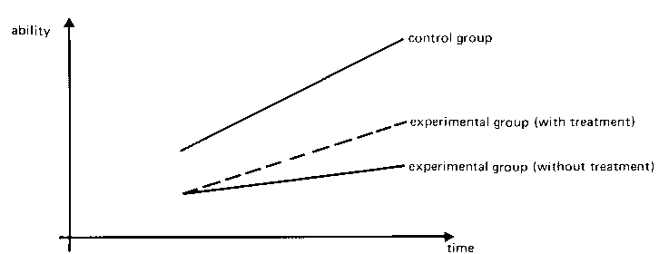
To illustrate the consequences of differences in initial rates of change, consider an example in which the experimental treatment is administered to the group developing
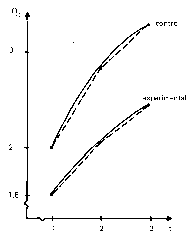
at the slower rate, with the other group used as a control group. In this case, the treatment could have a positive effect in increasing the rate of change of the experimental group, yet the actual change may not be as great as that observed in the control group. This kind of situation is depicted in Figure 1 in which the experimental treatment clearly has an effect, but which a traditional analysis of change scores would not reveal.
|
|
| FIGURE 1 Hypothetical Situation in which the Treatment has the Effect of Increasing the Growth Rate in the Experimental Group. |
To study the effects of treatments on rates of change, initial rates of change, and not simply initial statuses, are required. Therefore, because measurements at two points are required to estimate a rate of change, it is necessary that, in addition to a pre-test immediately before the introduction of any experimental treatment, even before that, another testing time be conducted. Thus it is necessary to have measurements on three occasions and not simply two.
While measurement at three time points may be necessary to evaluate both the initial rate of change and any change in that rate of change because of experimental intervention, this perspective on rate of change exposes another potentially important problem. The problem is the assumption that the rate of change is a linear function of time. This is most unlikely, and if change-rates, independent of treatment effects, are different, then comparisons which assume a linear change-rate could produce misleading results. To provide a simple analogy: consider the increase in weight of children where an increase of five pounds in weight for a five week old baby means something different from an increase of the same amount of weight in the same amount of time for a five-year-old child.
LINEARIZATION OF CHANGE: A META-METER FOR THE MODE OF CHANGE
An attempt to overcome the above problem of rates of change at different times can be made by using a rationale and model suggested by Rasch (1977). This model was developed independently of Rasch's SLM for test items, but it has the similar feature of structural invariance of parameters which characterizes that model.
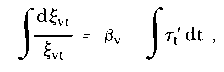
For convenience, suppose the variable considered is some ability, represented as a variable by the parameter ξvt for person v at time t. Now consider that the rate of change of ξ, dξvt/dt, is
(i) proportional to the current value ξ at time t, i.e.,
ξvt,
(ii) proportional to some parameter βv
characterizing person v, and assumed constant over time, which
might be called the person's individual change rate (with respect
to the given variable), and
(iii) proportional to some function of time τt',
which characterizes the change in this variable, is common to all
persons to be studied, and might be called the change mode
of the variable.
These relationships may be formalized according to
| dξvt/dt = ξvt βv τt | (1) |
This differential equation has a solution given by
| |
| ln xi;vt = αv + βv τi. | |
where αv is the constant of integration. Replacing ln ξvt by θvt, a new metric is created in which
| θvt = αv + βv τi. | (2) |
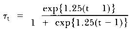
Equation (2) shows that at any time t, the ability of person v, θvt, depends on two person parameters, an `initial status' αv and a change rate βv. Furthermore, the ability θvt is linear in the variable characteristic, τt, which Rasch (1977) has called a `growth mode', which Rao (1958) has referred to as a `meta-meter', and which will be called the `change mode' throughout this article.
A significant feature of the change mode parameter is that it does not have to be linear in time. It is a change function which captures the nature of change for all persons considered appropriate to compare on this particular variable. Rasch used the model of equation (2) to analyze the weight changes of pigs while Rao, based on lectures given by Rasch, used it to study the weight changes of rats and babies.
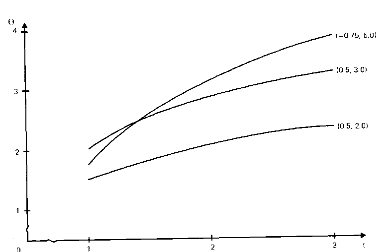
To illustrate some hypothetical change curves, the sigmoid change function
| (3) |
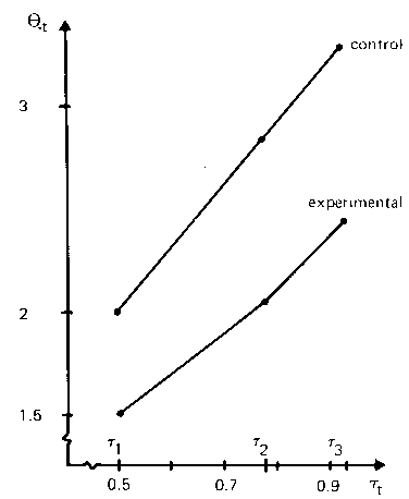
was used to generate three person change curves. The initial and change parameters (αv, βv) for the three persons were set at (0.5, 2.0), (0.5, 3.0) and ( -0.75, 5.0), respectively. The change curves are shown in Figure 2. It is apparent from Figure 2 that the comparison of change rates between any two persons at the same time, or between different times for the same person, may be misleading because of the lack of linearity of change over time. The change curves of the same three hypothetical persons, in the τ-mode, are shown in Figure 3. Clearly, the same change rates, and comparisons, would be inferred between persons, irrespective of the time points chosen.
|
| FIGURE 2 Growth Curves of Three Hypothetical Individuals in the Original Time Metric with Location and Growth Constants (αv, βv) Shown. |
|
|
| FIGURE 3 Growth Curves of the Same Three Hypothetical Individuals in the Meta-Meter. |
An important aspect of the change mode parameter for data analysis is that it can be estimated easily at each of the time points. Over a sample of N individuals,
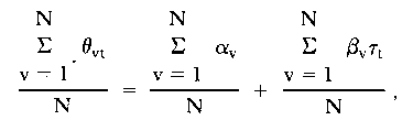
|
written as θ.t = α. + β. τt ,
can be, used to estimate τt. The normalizing constraints, α. = 0 and β. = 1, necessary to identify the parameters, provide the estimate
| τt (hat) = θ.t . | (4) |
With a large number of individuals, τt may be considered to be relatively well estimated by (4) and it is then possible to estimate αv and βv for each person.
However, the estimates of person parameters will not be made here. Instead, the case of two groups with different initial mean abilities will be pursued to indicate a way of testing the hypothesis that a treatment has had an impact on the rate of change.
Before proceeding, it is worth noting that Bryk, Strenio and Weisberg (1980), also propose estimating the amount of change that would occur independently of any treatment effect. The procedure, and the one considered here are not mutually exclusive. Indeed, one could use children's ages as a further variable in an elaborated model. Alternatively, the person parameter estimates, αv and βv may be seen to absorb any individual differences due to age. However, in the example to be considered below, the differences among individuals within groups in α and β are treated as error.
FORMALIZING COMPARISONS OF RATES OF CHANGE
Suppose then that there are two intact groups available to study the effect of some treatment and that three tests have been administered at different times. For purposes of notation, the control and experimental groups will be distinguished by superscripts C and E respectively.
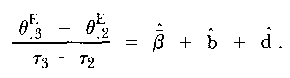
Parameterizing the model for groups
In general, we take the ability of each person at time t to be θvt and this includes various error components in change and in measurement. At time t = 2, θvt is given by θvt = θv1 + βv (τ2 - τ1), since αv is constant. While there may be in general fluctuations in the personal change rate parameter βv by the time of the second measurement it would not be possible to separate the stable and error components in βv and therefore no error component is shown between t = 1 and t = 2. However, to indicate the further possible fluctuations between t = 2 and t = 3, the change rate of person v will be parameterized as βv + εv where εv is assumed normally distributed with mean 0 and variance σ2ε. In the present situation, such fluctuations are considered to absorb the measurement errors. Then at time t = 3, θv3 can be expressed as
| θv3 = θv3 + (βv + εv) (τ3 - τ2) |
In addition to this general specification, suppose that the treatment is introduced at time t = 2 for the experimental group and that the potential effect of this treatment is to increase the personal change rate of each member of this group by an amount δv. Then for this group,
| θv3E = θv3E + (βv + δv)E (τ3 - τ2) |
where δv is now assumed normally distributed with mean δ- and variance of σε2 where, of course, δ- may or may not be zero.
This new change rate could alternatively be expressed as
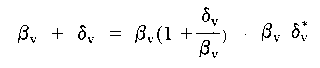
|
where the impact of the treatment on the change rate parameter βv is expressed as a factor δ- *v of this change rate. Certain potential advantages result from such a multiplicative formalization, and these will be considered in a subsequent section. For the moment, however, the increment in change rate is expressed additively.
To make it obvious that the groups may differ in initial statuses and in initial rates of change, these parameters will be expressed as deviations from the mean values within groups, and it is assumed that these deviations are normally distributed. The values for the two groups at various time points are summarized in Table I in which the Latin counterpart of the Greek letter in the experimental group indicates by how much this group is different from the control group in the particular parameter. Thus the letter `a' indicates the difference in initial status, `b' the difference in initial growth rates, and `d' indicates the possible impact of the experimental treatment on the growth rate in the experimental group.
| TABLE I PARAMETERIZATION OF PERSON IN CONTROL AND EXPERIMENTAL GROUPS AT 3 TIME POINTS | ||
|---|---|---|
| t | Control (C) | Experimental (E) |
| 1 | ||
| 2 | ||
| 3 | ||
While it would generally be relevant to evaluate whether or not a and b are significantly different from zero, in this preliminary and introductory report, attention will be focussed on evaluating the parameter d - the increment in change rate for the experimental group.
Estimating the change mode parameter
Before proceeding to the evaluation of the significance of d, it is noted again that the mode parameter is estimated simply according to equation (4) where the average θ.t is taken across both groups.
Estimating and testing the significance of relative increment in change rates
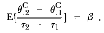
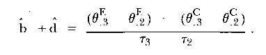
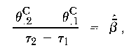
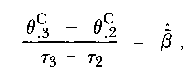
In order to prepare the way for the estimate of d, it is necessary to obtain first an estimate of the initial difference in change rates, b, between the two groups.
Within the control group
|
|
giving
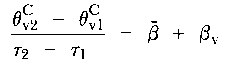
| (5) |
with
|
since, by definition,
|
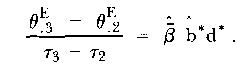
Analogously, in the experimental group,
|
|
giving
| (6) |
From (5) and (6)
| (7) |
Thus a mean value estimate b of b is obtained as
| (8) |
In an analogous derivation, it follows that
| (9) |
substituting for b^ from (8) into (9) and rearranging terms gives
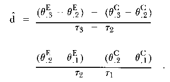
| (10) |
It should be noted that neither initial statuses, α, nor initial change rates, β, appear in equation (10).
To test H0:d = 0, it is necessary to have the variance of d (hat), or at least an estimate, V (hat) [d (hat)]. In deriving the variance, it is convenient to re-express the estimate, d (hat), in the form
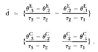
|
From some straightforward variance operations, it follows that
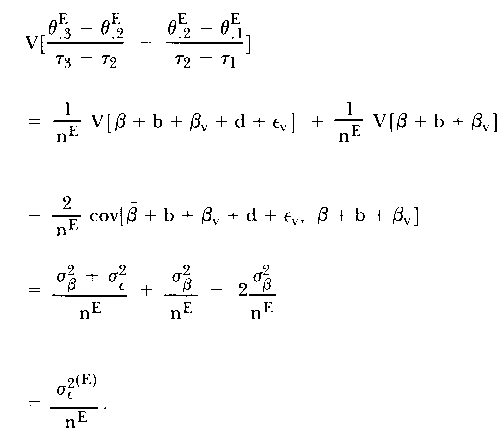
|
Analogously,
|
giving
| (11) |
which might be expected intuitively.
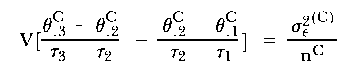
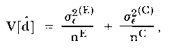
It seems that while V[d (hat)] has a straightforward expression, the best way of estimating it is to obtain estimates in each group of each of two variance components and the covariance component in the derivation of V[d (hat)].
Then the hypothesis H0:d = 0 can be tested using
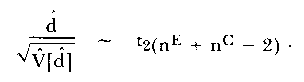
| (12) |
Unfortunately, neither the estimate of d (hat) nor the above statistical test is independent of the mode parameter, τ, since the differences τ3 - τ2 and τ2 - τ1 appear in the final expressions. Only in the unlikely case that τ3 - τ2 = τ2 - τ1 would they be eliminated.
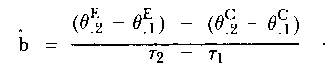
Estimating the change rate independently of the mode parameter
An estimate of the increment in change rate, d, can be made in such a way that it is independent of τ1. This is carried out by using ratios of differences rather than differences themselves, in the following way:
From (5),
| (13) |
and from (6)
| (14) |
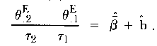
Now β- + b may be written as
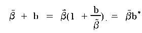
|
where now the increment in β with respect to the experimental group, which distinguishes it from the control group, is expressed as a factor b* of β- rather than as an addition to it. This gives
| (15) |
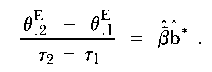
Forming the ratio of (15) and (13) provides an estimate of b* independent of the mode factor τ2 - τ1:
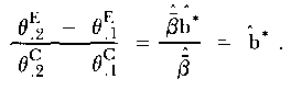
| (16) |
Analogously,
| (17) |
and
|
This time, β- + b + d may be converted to a product form according to

|
where now the increment in change rate at the second time point is expressed as a factor d* of the previous change rate βd*, rather than as an addition to it. This gives
| (18) |
Forming the ratio of (18) and (17) gives
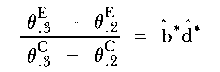
| (19) |
which is also independent of τ1. The ratio of (19) and (16) now gives the estimate of the increment in change rate of the experimental group
| (20) |
which again is independent of the mode parameter.
Unfortunately, at this stage, the estimate of the variance of d* seems somewhat intractable. However, because the estimate is free of the mode parameter, it is considered worthy of further study.
A SIMULATION STUDY
To illustrate an analysis of data according to the proposed model, a set of data was simulated so that the experimental group was initially at a lower status and changing at a slower rate than the control group. At the second time point, the experimental treatment was introduced and the experimental group increased its change rate, but the final change rate was still not as great as in the control group. The values of the parameters were chosen so that, with the given amount of error variance, the difference in change rates between the experimental and control groups would be just significant at the 2 1/2 per cent (one-tail) level of significance, that is, t = 1.96. The generating values of the parameters are shown in Table II. Two cases, one of sample size n = 30 and one of n = 50, are considered. A graphical representation of the parameters is shown in Figure 4, while a representation in the metric of transformed time, the mode parameter τt, is shown in Figure 5.
 |
 |
| FIGURE 4 The Status of the Experimental and Control Groups at Three Equally Spaced Times. | FIGURE 5 The Status of the Experimental and Control Groups at Three Times in the Meta-Meter. |
| TABLE II THE GENERATING VALUES FOR THE EXPERIMENTAL AND CONTROL GROUP MEANS AND VARIANCES AT THREE TIMES IN NON-LINEAR MODE FUNCTION | |||
|---|---|---|---|
| n = 30 | n = 50 | ||
| Control | θ.1C = 2.0 | 2.0 | |
| σαC = 0.988 | 1.276 | ||
| β.C = 3.0 | 3.0 | ||
| σβC = 0.988 | 1.276 | ||
| σεC = 0.988 | 1.276 | ||
| Experimental | θ.1E = 1.5 | 1.5 | a = -0.5 |
| σαE = 0.988 | 1.276 | ||
| β.E = 2.0 | 2.0 | b = -1.0 | |
| σβE = 0.988 | 1.276 | ||
| σεE = 0.988 | 1.276 | d = 0.5 | |
It is clear from the graphs that a traditional analysis of means at only the last two time points would show that the experimental group had not improved as much as the control group. However, in the context of the first time point, t = 1, which permits a study of initial relative rate of change, it is equally clear that the experiment did have a relative impact in incrementing the rate of change in the experimental group. This is particularly clear in the graph of Figure 5 which is displayed in the mode function.
Each of the simulation sets with n = 30 and n = 50 was replicated 20 times. The basic results of the significance test for H0: d = 0, as well as an estimate of the effect of d in terms of a factor d* of the rate of change β* are shown in Tables III and IV respectively.
The initial concern in examining the statistics of Tables III and IV is the correctness of the decisions that would be made. In this case, an incorrect decision is a Type II error-accepting a false null hypothesis. The expected number of correct decisions concerning these hypotheses can be obtained from the power of each test using tables in Winer (1971: 884) under the assumption that each distribution in fact is a noncentral t-distribution with the appropriate degrees of freedom shown in Tables III and IV and with non-centrality parameters equal to the `actual' values reported in those tables. The results of a comparison between the observed and expected number of correct decisions are shown in Table V.
| TABLE III RESULTS FROM 20 SIMULATIONS WITH n = 30 AND H0:d = 0 FALSE | ||
|---|---|---|
| Run No. | td (df=116) | d* |
|
1 2 3 4 5 6 7 8 9 10 11 12 13 14 15 16 17 18 19 20 |
5.293 1.482* 1.526* 3.241 1.098* 5.091 2.257 4.532 3.597 4.153 1.996 2.762 2.496 2.069 1.865* 2.978 5.331 1.999 1.612* 2.148 |
1.4975 1.1924 1.1371 1.3950 1.1195 1.4589 1.2078 1.5254 1.2854 1.3397 1.1986 1.3515 1.2168 1.2481 1.1042 1.2457 1.4124 1.2223 1.1454 1.2192 |
| Mean | 3.025 | 1.2761 |
| Variance | 2.780 | 0.0161 |
| Actual Value | 1.960 | 1.2500 |
| * Asterisked t-statistics refer to those leading to an incorrect decision about H0 with α = 0.025 (one-sided tests). | ||
These results show that in the case of n = 30, too many correct decisions were made. The source of this effect is provided in Table III in which it is evident that the mean of the t values is somewhat larger than it ought to be: 3.025 rather than 1.960. The variances of the t's also seem too large. These deviations may be due to the sample size, but they may also be affected by the presence of the values of the mode parameter in the test statistics.
| TABLE IV RESULTS FROM 20 SIMULATIONS WITH n = 50 AND H0:d = 0 FALSE | ||
|---|---|---|
| Run No. | td (df=116) | d* |
|
1 2 3 4 5 6 7 8 9 10 11 12 13 14 15 16 17 18 19 20 |
2.881 1.866* 1.483* 1.510* 0.693* 2.264 1.786* 3.796 1.102* 3.715 4.573 1.922* 0.616* 1.851* 2.120 1.478* 1.517* 3.400 1.484* 4.664 |
1.3140 1.1254 1.1074 1.1610 1.0796 1.2109 1.1861 1.3371 1.1032 1.3093 1.3568 1.1268 1.0318 1.1510 1.1753 1.1670 1.1755 1.2502 1.1916 1.3230 |
| Mean | 2.254 | 1.1941 |
| Variance | 1.449 | 0.0086 |
| Actual Value | 1.959 | 1.2500 |
| * Asterisked t-statistics refer to those leading to an incorrect decision about H0 with α = 0.025 (one-sided tests). | ||
| TABLE V OBSERVED AND EXPECTED NUMBER OF CORRECT DECISIONS REGARDING H0 : d = 0 WHEN H0 FALSE | ||
|---|---|---|
| H0: d=0 | n=30 | n=50 |
| Observed Expected |
15 9.8 |
8 9.9 |
For completeness, and because they do not involve the mode, it is worth noting the values of d*. These compare favorably with the actual value, and have a small variation. As explained earlier, no theoretical variance of these ratios has been derived. In practice, a jack-knife procedure may perhaps be used to obtain an estimate of this variance.
SUMMARY AND DISCUSSION
The study of the change of individuals seems central to many areas of concern in education and psychology. Despite considerable advances however in psychometrics, the interpretation of change on educational and psychological tests between two occasions by the same people continues to be difficult. With respect to the comparison of change among groups, of particular concern are the relationships between initial status and the change, especially in situations where initial statuses among groups are different.
It has been argued in this article that the continued concern with differences in initial status is intuitively based and that an explicit articulation of the reason why such concern continues should begin with an appreciation of why the initial statuses are different. For groups of the same average age, it is clear that the reason initial statuses are different is that the groups are changing at different rates. Therefore, it is suggested that if different treatment effects are to be compared by being administered to intact groups with different initial statuses - a situation often unavoidable in educational research - then initial rates of change, and not simply initial statuses, first need to be estimated. An exploratory simulation study was used to demonstrate one possible approach to such a design, and it has been shown that at least three occasions for the measurement, and not just two as in a pre-test and post-test design, are required.
Beyond the simple methodological and statistical problems, or perhaps underpinning them, a more important substantive point is revealed by the above considerations. This is concerned with the appreciation that if persons of the same age, categorized in some way or another into groups, are different in status on any criterion which may involve a change, then these persons must be changing at different rates. If this differential development has been proceeding for a number of years, say five or so, then it is unreasonable to expect that a special educational treatment of a group for a short period of time, and in the context of the many other factors continuing to impinge on the group, can increment the change of that group so dramatically that actual changes are very different from those observed in other groups. Perhaps the best that can be expected is that such a treatment may alter the direction of change, and, in the case of an identifiable useful single variable, the rate of that change. Continued exposure to the treatment for a substantial period of time may, by altering the rate of change have a large eventual impact on the final status of a person. However, in the short term, it is suggested that the most that can be observed is a comparison of where a group is after treatment relative to where it might have been without the treatment, rather than a direct comparison of the status with some other groups which might be changing at some general rate.
REFERENCES
Bryk, A. S., J. F. Strenio, & H. I. Weisberg, A Method for Estimating Treatment Effects When Individuals are Growing. Journal of Educational Statistics, 5, 5-34, 1980.
Cronbach, L. J. & L. Furby, How We Should Measure 'Change' - or Should We?, Psychological Bulletin, 74, 68-80, 1970. (And Errata, Psychological Bulletin, 74, 218, 1970).
Fischer, G. The Linear Logistic Model as an Instrument in Educational Research, Acta Psychologica, 37, 359-74, 1973.
Fischer, G. Some Probabilistic Models for Measuring Change. In De Gruijter, D. N. M. & L. J. Th. van der Kamp (eds), Advances in Psychological and Educational Measurement, London: John Wiley, 97-110, 1976.
Rao, C. R. Some Statistical Methods for Comparison of Growth Curves, Biometrics, 14, 1-17, 1958.
Rasch, G. Probabilistic Models for Some Intelligence and Attainment Tests, Copenhagen: Danmarks Paedagogiske Institut, 1960. (Reprinted, University of Chicago Press, Chicago, 1980.)
Rasch, G. On Specific Objectivity: An Attempt at Formalizing the Request for Generality and Validity of Scientific Statements, Danish Yearbook of Philosophy, 14, 58-94, 1977.
Stanley, J. General and Special Formulas for Reliability of Differences, Journal of Educational Measurement, 4, 249-52, 1967.
Winer, B. J. Statistical Principles in Experimental Design, 2nd ed., Tokyo: McGraw-Hill Kogakusha, 1971.
Wright, B. D. Solving Measurement Problems with the Rasch Model, Journal of Educational Measurement, 14, 97-116, 1977.
Wright, B. D. & M. H. Stone, Best Test Design. Chicago: MESA Press, 1980.
The Measurement of Change as the Study of the Rate of Change, Barry V. Kissane
Education Research and Perspectives, 9:1, 1982, 55-72.
Reproduced with permission of The Editors, The Graduate School of Education, The University of Western Australia. (Clive Whitehead, Oct. 29, 2002)
Go to Top of Page
Go to Institute for Objective Measurement Page
| FORUM | Rasch Measurement Forum to discuss any Rasch-related topic |
| Coming Rasch-related Events | |
|---|---|
| May. 15 - June 12, 2026, Fri.-Fri. | On-line workshop: Rasch Measurement - Core Topics (E. Smith, Winsteps), www.statistics.com |
| June 19 - July 25, 2026, Fri.-Sat. | On-line workshop: Rasch Measurement - Further Topics (E. Smith, Winsteps), www.statistics.com |
| Aug. 31 - Sept 2 2026, Mon.-Wed. | In person: IMEKO TC1 Metrology Education and Training symposium, Klagenfurt, Austria www.photomet-edumet2026.com. Submissions by April 20 |
| Aug. 30 - Sept. 3, 2027, Mon.-Fri. | In Person: 2027 IMEKO World Congress (TC1, Tc7, TC13, TC18, TC26), Rimini, Italy imeko2027.org |
Our current URL is www.rasch.org
The URL of this page is www.rasch.org/erp5.htm