
The correspondence between a data set and a statistical model defines the notion of `fit'. In psychometric models of the Rasch class, all aspects of fit cannot be judged from a single statistic. On the other hand, all that can be learned about the fit of data to a Rasch model must be contained in the residuals or magnitudes of departures from the model. Various tests based directly on these residuals are reviewed.
INTRODUCTION
A key aspect of science development is the construction and verification of correspondence between observed data and an abstract model designed to represent the data. Modern psychometrics employs statistical models (taking the form of probability distributions), to describe, more or less, the results of mental tests. The degree of correspondence between empirical observations and those predicted through the operation of the model is generally known as `fit between the data and the model'.
The utility of the results of measurement in the social sciences rests to a large extent on a judicious choice of model. An investigation of the degree of fit is essential since conclusions are derived through the model properties and specifications and not directly from the particular observed data. For example, in the analysis of items within a test, it is the item difficulty parameter that is of major importance, not the specific set of observations which might lead to one particular estimate of that parameter. The purpose of using a model is thus to replace any particular data set with the more general model. The confidence in this replacement rests in part on the psychometric tests of fit.
Models are not expected to predict outcomes perfectly according to every conceivable criterion of accuracy. It is the degree of correspondence between data and model which is tolerable in terms of utility for a given purpose, which determines ultimately the extent of `fit of data to the model'. Thus any particular test of fit between a data set and the model is never complete.
To put it another way, the decision actually to use measures depends not only on their quality according to psychometric criteria, but also on non-psychometric factors such as economics, time restrictions and politics. This latter point is emphasized since recent articles (Gustafsson (1980), van den Wollenberg (1981)), appear to ignore this fundamental issue when reporting fit or when they criticize the statistics proposed to indicate degree of fit.
An aim of the following discussion is to draw a balance between the two extreme approaches to the relationship of test data to statistical models which are supposed to describe those data. On the one hand there is the point of view which sees the collected data as sacrosanct. Hence if a given data set does not fit the originally proposed model, one is expected to change or modify the model, most often by including further parameters to account for patterns in the data, or by deleting some parameters because they are superfluous.
On the other hand, there is the point of view that the model is `perfect'; it is usually argued on logical and/or measurement principles that the nature of measurement should comply with certain fundamental axioms and from this stance one establishes the necessity of a specific model. Since the model is argued on these grounds, it is the data which must be manipulated if there is any evidence of lack of fit. Most practitioners work somewhere between these two extremes, although those who advocate Rasch models tend to work towards the latter framework whereas those who work with the models of Lord and Birnbaum (1980), tend to work from the former framework.
It is worth noting that when it is the data which must be edited in some way, tradition has it that items and not persons need attention in order to enhance fit. Recent arguments center on a more symmetrical approach to fit via the analysis of misfitting persons as well as misfitting items. There is a sense in which the adoption of these psychometric models by mathematical statisticians has resulted in a lessening of importance attached to the work contributed by practicing psychometricians. It is for these reasons and the fact that an increasing variety of `tests' are being proposed for at least one large class of models that this article has been written; the discussion has been restricted to the class of models known as Rasch models since little work on fit has been forthcoming with respect to other models. These points are illustrated by the various tests of fit described in this article.
THE STATISTICAL ASPECTS OF FIT
It is informative to describe in some detail the way in which statisticians generally test the fit between data and discrete probability distributions from primarily a statistical point of view. The following description is necessarily simplified but does capture the essential logic. In the first instance, the probability distribution (i.e., the model), must be fully specified; that is, the algebraic form, the parameter(s) and the sample space of possible events must be stated. 'Fit' is the correspondence, then, for a given set of real data of sample size N, between the observed frequencies (of each element of the sample space) and those frequencies predicted by the particular model. There are various ways of calculating the 'correspondence'.
| TABLE I | ||
|---|---|---|
| x | nx | E[nx] |
| 0 1 2 3 4 4+ |
109 65 22 3 1 0 |
108.7 66.3 20.2 4.1 0.7 0.0 |
| λ (hat) = 0.61 | ||
The basics of fit from the common statistical viewpoint will be illustrated by reference to the often quoted data set arising from records kept of the number of deaths by horse-kick in the Prussian army and analyzed via the discrete Poisson distribution by Bortkiewicz (1898). In these data, there were ten army corps which were sampled each over 20 years, giving N = 200. The relevant data and calculations for fit appear in Table I, where x is the number of deaths and nx, is the number of army corps with x number of deaths.
The Poisson model states that:
| (1) |
where the parameter of the model, λ, is estimated (maximum likelihood or otherwise) from the data. The estimated probability of each event, px (hat), can be found by substituting λ (hat) for λ. Then an estimate of the expected value is found from E[nx] (hat) = Npx (hat) [where (hat) means "estimated from the data"]. The observed and expected nx columns may be compared for correspondence, usually by some form of Chi-square statistic. It is also possible to calculate raw residuals for these data, that is, the difference between a single specified observation and its expected value. This is given by
| X - E[X] = X - λ | (2) |
An estimated residual is found by substituting λ (hat) for λ. There are as many residuals as there are observations, in this case, 200. For example, if in 1880 in army corps A the number of deaths was two, then the residual for that observation would be 2 - λ (hat) = 2 - 0.61 = 1.39. Residuals for these data range from -0.61 to 3.39.
In order to illustrate a point which arises frequently in the discussion of fit to psychometric models, we note that there were four deaths in one army core. On the basis of these data the Poisson model, and the sample size of 200, it is not surprising that there was one army corps with four deaths in one year. It certainly would be concluded that the four deaths are in accord with the model and in fact the standard test of fit applied to these data results in an affirmation of fit which is so good that some statisticians have raised questions of 'over-fit'. However, horse deaths are rare events, and to have four of them in one year in one army corps might suggest an examination of that army corps. Perhaps a new captain was somehow implicated, or all four people were killed by the same horse or some other empirical explanation may be hypothesized why this particular corps had four deaths.
If a global test of fit is the limit of investigations, failure to understand important aspects of the data may occur; the purpose of fit is not just to make a simple 'yes' or 'no' declaration that the model and data accord, but to have a greater understanding of the way in which the data arose. This perspective has led practitioners to think in terms of 'psychological' fit in addition to statistical fit. These notions will be elaborated in the next section.
FIT AND THE RASCH MODEL
The fit-logic from a statistical point of view is now applied to the model of Rasch (1960, 1980). The probability distribution has the algebraic form
| P{X;βv,δi} = exp[(βv - δi)X/{1 + exp[βv - δi]}, X = 0,1 | (3) |
in which there are two parameters and two points in the sample space. Because there are only two outcomes, this distribution describes a Bernoulli random variable. To estimate the two parameters, it is necessary to have replications. It is impossible, however, to replicate the observations without introducing certain types of dependency conditions so that the standard statistical rules for IID [identical independently distributed] random variables would not apply. Thus each person v generally answers more than one item to provide 'pseudoreplications'; so for person v there is a compounding of Bernoulli random variables, but because each item has a different difficulty parameter, the distributions are not identically distributed.
Despite these complications a genuine probability distribution arises if, with L items, the probability of the response pattern, (X1, . . ., XL.), is derived. This probability, after suitable algebraic manipulation, is written as
 | (4) |
In practice, at least for an item calibration exercise, an even more complicated version of the model is dealt with, since the probability distributions are simultaneously replicated over a sample of persons. In practice, the probability distribution is stated as if the number of items were fixed at L. This permits an interpretation whereby N (the number of persons tested) has the same connotation as it did with the horse-kick data. Hence
 | (5) |
with the sample space of possible events equal to the 2L potential patterns of responses. The sample size is N and there are N + L parameters (questions of identifiability and independence of parameters are ignored for the present).
The data in Table II below are fictitious but serve to highlight some of the problems regarding fit. They describe the response patterns of N = 300 persons taking an L = 3 item `test'. It is assumed that the item parameters are known with δ1 = - 1.0, δ2 = 0.0, δ3 = 1.0, and that all 300 subjects have the same ability βv = -1.0.
| TABLE II ILLUSTRATIVE RASCH DATA | ||
|---|---|---|
| (Xv) | Nx | E[Nx] |
| (100) (000) (110) (010) (101) (111) (001) (011) |
153 58 54 19 9 3 3 1 |
151.89 56.16 56.16 20.79 7.98 2.97 2.97 1.08 |
| 300 | 300 | |
It is possible to provide a residual in the form of a vector of observed responses versus predicted responses. Since
| E[(Xv)] = (E[Xvi]) = (pv1, ..., pvL) | (6) |
(X1, ..., XL) is compared with (p1, ..., pL), to obtain a vector of residuals for each observation. For example, 153 persons scored (100); that is, these 153 persons had only the easiest item correct. The residual vector for any one of these persons (all of them have the same ability of -1.0), is
(1 0 0) - (.73 .27 .05) = (.27 -.27 -.05).
Now consider the three persons with the pattern (001). These three persons had only the hardest item correct, and the residual for each of these three is
(0 0 1) - (.73 .27 .05) = (-.73 -.27 .95).
The point illustrated in the above example has been somewhat labored in order to make a distinction between attention to the psychological (or process) model and the statistical model; some events acceptable under the statistical model are psychologically questionable and a thorough analysis of the data would warrant an investigation of the reasons why even one person had such a peculiar answer pattern since ultimately the question will be asked whether or not this person had been measured on the construct of interest.
TESTS OF FIT FOR THE RASCH MODEL
In the succeeding sections the various suggestions that have been made with respect to fit of data to the Rasch model are discussed. Although an exact chronological order will not be observed, some attempt will be made to demonstrate the historical development of fit idea. Since the first papers dealing with this topic were published there have been disagreements regarding the 'correct' degrees of freedom, the extent of bias in the fit statistics, the use of conditional (CMLE) or unconditional (JMLE) probabilities, and so on. Such debates on statistical criteria for fit are still popular in both the published literature and at major psychometric conferences.
It is the contention of this writer, however, that for the analysis of fit of most sets of real data (in which at least 12 items form a test), the arguments for one statistic versus another lose their impact. For example, van den Wollenberg (1981) claims that the Wright and Panchepakesan [WP] statistic (1969) is 'heavily at fault'. However, for data from tests of 12 or more items, van den Wollenberg's 'new' statistic, Q1, which tests the same violation of the model as the Wright and Panchepakesan statistic, is indistinguishable from it. Similar features can be demonstrated among other competing statistics.
It seems more profitable, therefore, to concentrate on procedures which genuinely differ in principle from one another.
Rasch (1960, 1980) used the term 'control of the model' to describe what has been called 'fit of the model'. In his mathematical development of the model via conditional probabilities, the pertinent probability distribution is the conditional distribution of response pattern conditioned on the sufficient statistic (which is the raw score arising from the pattern). Obviously many different patterns lead to the same raw score. The probability of each of these patterns, conditional on that raw score rv is given by
 | (7) |
in which the γrv are elementary symmetric functions of the item parameters, (δ). A double conditioning of the total data matrix leads to
| p{((Xvi))|(r), (S)} = 1/C | (8) |
in which (S) is the vector of item counts, (r) is the vector of N raw scores and C is a combinatorial number (the number of different 0/1 data sets which could produce the marginals (S) and (r)). Rasch says that this probability serves as a 'basis for parameter-free controls of the model'; since no estimation of parameters is required, exact tests of fit (in the sense of R.A. Fisher), are forthcoming. Rasch himself however, was quick to realize the near impossibility of determining C and to date no-one has been able to follow up those suggestions. [With modern computer-power this could be done, but it would serve no real purpose.]
As a result of the practical problems with the parameter-free tests, Rasch suggested approximations based on the observed proportions Sgi/Ng of the number of persons in score group g who had item i correct, such that the ratio Sgi/(Ng - Sgi) could be used in score group g to estimate exp(βg - δi). Rasch suggested that the proportions be used as a basis for a test of fit by looking at the G = L - 1 different estimates. He suggests plots both for groups of items (grouped by their difficulties) and by persons (grouped by their raw scores). Wright (1967) elaborated on these plots and gave added insight into their utility for determining fit. There is a very real sense in which all tests of fit to the Rasch model which have been proposed in the last 20 years are simply variations of these original suggestions.
In 1969 Wright and Panchepakesan described a more formal test of fit based on the notions of splitting people into exclusive groups. Repeated reference and use of this statistic has led to its naming as the WP statistic. Persons are split into G groups on the basis of their raw scores and the observed number in each group with each item correct, Sgi, is compared to the expected number, the latter arrived at via the model after all item and person parameters have been suitably estimated. This comparison between observed and expected statistics may be accumulated over items to produce a total WP statistic. It is noted that the WP procedure uses unconditional (JMLE) probabilities for determining pvi.

| (9) |
Formal significance testing may be carried out by noting the approximate Chi-square distribution of WP in practical testing situations. As noted earlier, van den Wollenberg's Q1 statistic (1981) is equivalent to WP when more than 12 items are involved.
In the early 'seventies a modification of the WP approach was proposed by two groups of people on either side of the Pacific. In Austria, Fischer and Scheiblechner, and in the USA, Wright and colleagues, suggested that instead of predicting expected frequencies via the model, the item difficulties should actually be re-estimated in each group upon which the split had been made. The program MLTBIN of Andrich (1975) uses a median split although there is no logical barrier to a split based on G groups. The test of fit is an application of a statistical test of the homogeneity of a number of estimates of a model parameter and is described fully in Rao (1973). The statistic admits of an interpretation both for each item and for the collection of all items as a whole. The statistic Hi is given by

| (10) |
in which the pooled estimate of the item difficulty is

| (11) |
and its variance is

| (12) |
Hi, which is distributed as Chi-square on G-1 df, may be accumulated over i to form a global test. Asymptotically this test has a similar distribution to that of WP.
A likelihood-ratio test was devised by Andersen (1973); it used as its guiding principle the logic outlined for the Fischer/Scheiblechner approach. Instead of adopting the Rao test, Andersen formed the (conditional) likelihood of the data based on the overall item estimates and also the (conditional) likelihood of the data for each subgroup. Thus

| (13) |
was shown to be Chi-square, in which

| (14) |
This test follows in the spirit of maximum likelihood estimation; it is noted that a similar LR test could be devised on the basis of the unconditional (JMLE) likelihoods and some recent developments of Rost (1982, this issue), demonstrates the power and utility of such an approach. However, because there is no sensible partitioning of the Chi-square statistic LR tests of any description give us no information about aberrant items. For this reason they provide little practical advantage. We may further note that the LR test is asymptotically equivalent to the WP statistic so in one sense WP, Q1, H and LR will all lead to similar conclusions about a given data set - whether instituted conditionally or unconditionally.
In a slightly different context, Leunbach (1976) devised various tests of the hypothesis that two mental tests measure the same variable. The tests adhere to Rasch's principles in that they arise out of a conditional argument and lead to a probability distribution of the general form

| (15) |
in which (δ(1)) and (δ(2)) are the two sets of item estimates and for which the sufficient statistics are marginals of the number of persons, nr1r2, with various combinations of raw scores (on each of the tests and in which the actual person parameters have been eliminated as usual by the conditioning). Since relatively extensive data sets are required to ensure that no nr1r2 are zero, the tests appear to have limited practical application in their present form.
Another innovation from 1976 may be found in the dissertation of Mead and later resurrected by Divgi (1981). It is based on well-known principles of simple linear regression and indirectly provides an estimate of the slope of an item's characteristic curve. Some psychometricians refer to this property as the item's discrimination and actually parameterize it in their models. Working from general linear model theory, Mead postulated that a residual for person v on item i, written

| (16) |
may be further explicated in terms of the linear form
| yvi = a0i + a1ibv + a2ibv2 , | (17) |
where (i) a0i is zero if the group of persons involved is actually the calibration group (otherwise a0i acts as a `difficulty shift'),
(ii) a1i, the linear coefficient, is the index of item discrimination, and
(iii) a2i, the quadratic coefficient, relates the extent of `guessing' or 'indifference'.
A formal test of fit would proceed as an analysis of variance with the nullity of a2i considered first, and upon acceptance of that hypothesis, the nullity of a1i also investigated. Fit to Rasch model is claimed when the latter hypothesis is accepted also. It should be realized that these tests of fit, directed as they are to quite specific hypotheses, are relatively powerful when compared with the more global tests considered previously (there are far fewer degrees of freedom to account for), but on the other hand are likely to be less powerful for detecting departures arising from factors unrelated to guessing and varying discriminations. Perhaps Mead's major contribution was his application of an identical argument to the derivation of a test of `person fit', based on the same residuals yvi, in which case
| yvi = a1vdi + a2vdi2 , | (18) |
Hence the test of a person's `linear fit' is contingent upon the nullity of a2v.
The term `person fit' has been coined to describe those Rasch analysis activities which focus attention on aberrant patterns of responses for individuals taking a test. Aberrant patterns are those of very small probability, even though they might be `expected' in large enough samples according to the specification of a probability model. It is one thing to note that patterns of small probability will occur; it is quite another to realize that the patterns are created by persons taking tests and that a responsibility exists to investigate these situations since it is difficult to believe that such persons have been measured on the variable. A description of person-fit in practice is to be found in Wright and Stone (1979).
Most person-fit analyses calculate the probability of each person's response pattern and flag those of very small probability. Additional information is available for diagnosis if both observed and expected patterns are displayed in the analysis. For example, it is difficult for the psychometrician to believe, and even harder to explain, the observable fact that a person whose raw score is 2 obtained that score by answering correctly the two most difficult of 30 items-and still argue that the score of 2 represents as valid a measure on the variable as does the 2 of the person whose correct items are the two easiest on the test.
In practice the person-fit statistics used to highlight the misfit are some variations of the probability of the response pattern; most often they involve a summation over items of the person's standardized residuals and the conversion of this sum to a Chi-square or mean-square statistic with suitable distribution properties. For example, a person fit statistic used by Andrich (1980) has the following form:

| (19) |
where (i) 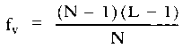 is the
degrees of freedom, and is the
degrees of freedom, and
| |
(ii) 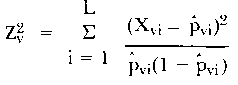 is the sum of squared residuals. is the sum of squared residuals.
| |
The purpose of the logarithmic transformation is to stabilize the variance of the statistic T so that it has an approximate normal distribution.
Some interesting variations on existing fit statistics and the exposition of a new statistic have been devised by two Europeans, van den Wollenberg (1981) and Molenaar (1981). Their arguments derive from the original work of Rasch and unpublished work of Martin-Löf. In order to understand the rationale of these tests, one needs to have a grasp of the differences between conditional (CMLE) and unconditional (JMLE) Rasch analysis. When Wright and Panchepakesan devised their WP statistic, they used the expected value of a response by person v to item i the unconditional probability
| P{Xvi; βv,δi} = pvi = exp[(βv - δi)X/{1 + exp[βv - δi]} | (20) |
Since responses by person v to a set of L items are statistically independent, the covariances, Cov[Xvi, Xvj] are zero, and thus play no part in the tests of fit. Most variations on the basic tests of fit, however, as devised by European psychometricians, rely on the conditional probability of the response, given the raw score rv. In this case the expected value has the form
| πri = exp[-δi]γr- 1,i/γr , | (21) |
and does not involve person parameters as does the unconditional form shown above. (γr-1,i and γr are elementary symmetric functions of the δ's only). Although even Rasch found it difficult to write out explicitly the bivariate distribution of Xvi and Xvj (given rv), it is not difficult to show that the covariance is given by

| (22) |
where γr-2,ij is also a symmetric function in all δ's except δ1 and δj. Clearly, the conditional responses are not independent and any test of fit should take this into account if the dependence is likely to play a part in the ultimate fit decisions.
Martin-Löf provided a formal test of fit which incorporates the covariances. His statistic, in matrix notation, is

| (23) |
where δ'g (hat) is the transpose of the g x 1 vector of difficulty estimates in group g, and Vg- 1 is the inverse of the covariance matrix of these estimates. Van den Wollenberg has also demonstrated that when all item estimates are considered equal (an equivalent items test), T approximates the WP statistic and is in fact algebraically identical to van den Wollenberg's conditional version of WP, the Q1 statistic. The most recent effort of van den Wollenberg and Molenaar (1981) has been to effect a compromise between the excessive computations of T and the approximate nature of Q1. The new statistic, Q2, builds upon 'second-order' frequencies and appears to be quite powerful as a test of dimensionality. For the group with score r, observed 2 x 2 tables are constructed as follows:
| ITEM i | ITEM j | ||
| Srij | Sri~j | Sri | |
| Sr~ij | Sr~i~j | Sr~i | |
| Srj | Sr~j | nr | |
where Sri~j, for example, means the number of people with score r who have item i correct and item j incorrect. These observed tables are to be compared with expected 2 x 2 tables in which the entries are obtained from

| (24) |
and in which item estimates have to be obtained from each score group r. The statistic Q2, summed over all score groups and all item combinations has an approximate Chi-square distribution; little evidence is available concerning its practicability with respect to real data.
A recent contribution of Molenaar (1981) has been the introduction of what he terms `splitter' items to test unidimensionality. The sample is split into two subsets, Gi+ and Gi-, of those who answered item i correctly and those who answered it incorrectly. After separate calibrations (in each group), of the remaining items, evidence of multidimensionality would be forthcoming when the items easy for Gi+ and hard for Gi- form one dimension and the reverse set the other dimension. WP (or Q1) would be determined for the two groups and a formal test of fit applied as often as liked to select different `splitters'. It would be informative as well to plot item estimates for Gi+ and Gi-.
CONCLUSION
The most valuable contribution to the area of tests of fit for Rasch models in recent years has been the recognition by some psychometricians that there is no such thing as a final `fit' of data to the model and hence that no one test is ever likely to be complete. Appreciation of this point still needs to be given much wider circulation among workers in the field. Then there will be less of a tendency to reject data sets (or the model) outright, simply because one test failed to show `fit'. Implicit in this perspective is the assumption that there is as much to be learnt about a data set from the responses which misfit as there is from those which do fit.
Issues in the Fit of Data to Psychometric Models, Graham Douglas
Education Research and Perspectives, 9:1, 1982, 32-43.
Reproduced with permission of The Editors, The Graduate School of Education, The University of Western Australia. (Clive Whitehead, Oct. 29, 2002)
REFERENCES
Andersen, E. B. A goodness of fit test for the Rasch model. Psychometrika, 1973, 38, 123-40.
Andrich, D. The Rasch Multiplicative Binomial Model: Applications to Attitude Data, Research Report Number 1, Measurement and Statistics Laboratory, Department of Education, University of Western Australia, 1975.
Bortkiewicz, L. V. Das Gestz der Kleinen Zahlen. Leipzig, Teubner, 1898.
Divgi, D. Does the Rasch model really work? Paper presented at Annual Meeting of the National Council on Measurement in Education, Los Angeles, 1981.
Leunbach, G. A probabilistic measurement model for assessing whether two tests measure the same personal factor. Unpublished paper, 1976.
Lord, F. M. Applications of Item Response Theory to Practical Testing Problems. Hillsdale, N.J.: Lawrence Erlbaum Associates, 1980.
Mead, R. Assessment of Fit of Data to the Rasch Model Through Analysis of Residuals. Unpublished Doctoral Dissertation, University of Chicago, 1976.
Molenaar, I. Some Improved Diagnostics for Failure of the Rasch Model. Heymans Bulletins Psychologische Instituten. R. J. Groningen, HB-80-482-EX, 1981.
Rao, C. R. Linear Statistical Inference and its Applications. (2nd ed.) John Wiley & Sons, N.Y., 1973.
Rasch, G. Probabilistic Models for Some Intelligence and Attainment Tests. (Copenhagen, Danish Institute for Educational Research, 1960), Chicago, University of Chicago Press, 1980.
van den Wollenberg, A. On the Wright-Panchepakesan goodness of fit test for the Rasch model. (In press), 1981. [Probably published in van den Wollenberg's 1982 papers.]
Wright, B. D. Sample-free test calibration and person measurement. Proceedings of the 1967 Invitational Conference on Testing Problems. Princeton, N.J.: E.T.S., 1967.
Wright, B. D. & N. Panchepakesan. A procedure for sample-free item analysis. Educational and Psychological Measurement, 1969, 29, 23-57.
Wright, B. D. and M. H. Stone. Best Test Design. MESA Press, Chicago, 1979.
Go to Top of Page
Go to Institute for Objective Measurement Page
| FORUM | Rasch Measurement Forum to discuss any Rasch-related topic |
| Coming Rasch-related Events | |
|---|---|
| May. 15 - June 12, 2026, Fri.-Fri. | On-line workshop: Rasch Measurement - Core Topics (E. Smith, Winsteps), www.statistics.com |
| June 19 - July 25, 2026, Fri.-Sat. | On-line workshop: Rasch Measurement - Further Topics (E. Smith, Winsteps), www.statistics.com |
| Aug. 31 - Sept 2 2026, Mon.-Wed. | In person: IMEKO TC1 Metrology Education and Training symposium, Klagenfurt, Austria www.photomet-edumet2026.com. Submissions by April 20 |
| Aug. 30 - Sept. 3, 2027, Mon.-Fri. | In Person: 2027 IMEKO World Congress (TC1, Tc7, TC13, TC18, TC26), Rimini, Italy imeko2027.org |
Our current URL is www.rasch.org
The URL of this page is www.rasch.org/erp3.htm