Rasch Lessons from the Netflix® Prize Challenge Competition

The Netflix Prize Challenge Competition ran for 34 months from October 2, 2006 until July 26, 2009. Netflix supplied a "Training" dataset of 100,480,507 ratings made by 480,189 Netflix clients for 17,770 movies between October, 1998 and December, 2005. The ratings were on a rating scale of one star to five stars. The Training data matrix has 99% missing data. Netflix also supplied a dataset of 2,817,131 "Qualifying" ratings. For these ratings, the clients and movies are known, but the actual ratings were known only to Netflix (until the competition concluded). The Netflix Prize was awarded to the team most successful at "predicting" those publicly unknown ratings. Teams were allowed to submit multiple prediction datasets.

Team "BellKor's Pragmatic Chaos" won the Prize in a tie-break based on a 20-minute earlier submission time of their winning prediction dataset. The runners-up were team "The Ensemble" (of which I was a member). The team that had the "dubious honors" (according to Netflix) of the very worst predictions, out of the 44,014 valid submissions from 5,169 actively participating teams, was team "Lanterne Rouge" of which I was the leading member. Of course, these worst predictions were deliberate!

During the 34 months of the Prize competition, there were some valuable lessons with general application in Rasch analysis.

1. Dataset size.

When stored as a rectangular text data-file, the size of the Training dataset is at least 480,189 * 17,770 bytes = 8,532,958,530 bytes = 8GB. When implemented in Winsteps, this required 8GB of input data file and two more work files of the same size = 24 GB (at least). But 99% of these 24GB are missing data. So this was highly inefficient. Simultaneously, Winsteps users were noticing the same thing for their computer-adaptive-testing (CAT) and concurrent-test-equating analyses. In contrast, the same data in Facets (for which missing data do not need to be stored) have an input dataset size of 1.3GB and a work file size of 0.6GB. So obvious improvements to Winsteps were to allow Winsteps to use a Facets-style input-data-format, and to use a compressed work-file algorithm. This reduced the Winsteps input dataset size to 1.3GB and the work-file sizes reduced to 3.3GB and 0.2GB, a total of 5GB instead of 24GB.

2. Processing time.

The first run of Winsteps on the Training dataset indicated that the estimation process would take 8 days to come to convergence. Consequently that first run was cancelled after 1 day as entirely impractical. The first run in Facets on the same data required about 24 hours. Again this suggested improvements could be made to Winsteps. Reducing the dataset disk-size also reduced the input-output overhead, so reducing processing time. But inspection of the computer code also revealed routines which could be made faster. Consequently Winsteps processing time was reduced to about 12 hours, and much less if only rough convergence is required.

3. Rasch Models.

Each time a dataset of predictions was submitted to Netflix, Netflix responded with a summary statistic on the accuracy with which the "Quiz" half of the qualifying ratings had been predicted. Competitors did not know which of the Qualifying ratings comprised the Quiz dataset. The other half of the Qualifying ratings were termed the "Test" dataset. The summary statistic for the Quiz dataset was the root-mean-square-residual (RMSR), called by Netflix the root-mean-square-error (RMSE), between the known-to-Netflix values of the ratings and their competitor-predicted values. The values of the RMSRs enabled competitors to know which of their prediction models were more effective. Netflix permitted submissions to included predictions between categories, such as 3.5674 stars. This improved RMSRs relative to predicting exact categories.

An immediate finding was that the Rasch-Andrich Rating Scale model (RSM), applied to the 5 category (1 star to 5 star) Netflix rating scale was more effective (RMSR= 0.9815) than either a Rasch-Masters Partial Credit model applied to the 17,770 movies (RMSR=0.9867) or to the 480,189 clients (RMSR=0.9907). Less parameters, but better prediction!

4. Pseudo-Rasch Dichotomous Fractional Model.

As the competition proceeded, it became apparent that the data were severely multidimensional, and that a unidimensional Rasch analysis was a useful first-stage leading on to other analyses. But, as implemented in Winsteps and Facets, the Andrich Rating Scale model requires the computation of 4 exponentials for each observation in each estimation iteration as well as the accumulation of probabilities for the five categories. Further the threshold estimates need to be brought to convergence. If this processing load could be lessened, without severely impacting the utility of the Rasch measures, then the duration of the first-stage Rasch analysis would be considerably reduced.

This motivated the "Pseudo-Rasch Dichotomous Fractional Model" (DFM). In the Rasch dichotomous model (DM), the observations are "1" (success) and "0" (failure). In RSM, the Netflix rating scale is modeled to be 5 qualitatively-ordered categories along the latent variable. In DFM the 5 categories are modeled to be predictions of the probability of success on a dichotomous item. 5 stars = 1.0 probability. 4 stars = 0.75 probability. 3 stars = 0.5 probability. 2 stars = 0.25 probability. 1 star = 0.0 probability. DFM simplifies and speeds up all the rating-scale computations to be those of the DM. In JMLE (as implemented in Winsteps and Facets), the parameter estimation converges when "observed marginal score ≈ expected marginal score" for all parameters. The expected marginal score is computed in the usual DM way. The observed marginal score is the sum of the prediction-probabilities (based on the Star ratings) for each parameter. The resulting DFM Pseudo-Rasch measures for movies and clients are effectively collinear with the RSM measures. The DFM model was implemented in special-purpose software [but can easily be implemented with Facets]. It achieved its objective of speeding up estimation without noticeably degrading prediction accuracy, relative to RSM.

5. Correction for extreme observations.

Since the Netflix criterion for accuracy of prediction was the RMSR, incorrectly predicting that an observation would be 1 or 5 Stars was considerably worse, on average, than incorrectly predicting that an observation would be in an intermediate category. The use of the extreme 1- and 5-Star categories by Netflix clients was somewhat idiosyncratic. An improvement to prediction resulted when the influence of the extreme categories was reduced. For the DFM model, experiments revealed that better inferences were obtained by substituting to 4.75 Stars (in place of 5 Stars) and 1.25 Stars (in place of 1 Star), and adjusting the probabilities accordingly. For the RSM model (as implemented in Winsteps), this is done by adjusting observed category frequencies. For 5 Stars, the observed rating-score was reduced from 5.0 to 4.75, and the corresponding observed category frequencies were changed from 1 observation of 5 into 0.75 observations of 5 and 0.25 observations of 4. Similarly for 1 Star.

6. Estimating RSM thresholds.

The estimation of RSM rating-scale thresholds has long been troublesome. The original JMLE technique, proposed in "Rating Scale Analysis" (Wright and Masters, 1982) estimated each threshold using Newton-Raphson iteration, as though it was an almost separate parameter. This technique proved too unstable when category frequencies were very uneven or there were pernicious patterns of missing-data. So Newton-Raphson iteration of the threshold estimates was replaced in Winsteps by "Iterative curve-fitting", because the relevant functions are known to be smoothly monotonic logistic ogives.

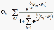
For the Netflix data, a faster-converging estimation method for rating-scales was sought. An iterative approach based on solving simultaneous linear equations has proved effective. Suppose that P_k is the expected frequency of category k in the dataset according to RSM.

where K_nij = B_n - D_i - F_j except that K_ni0 = 0. F_j is the Rasch-Andrich threshold at which categories j-1 and j are equally probable.

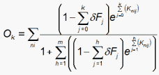
Suppose that a small change δF_j in F_j (and similarly for all the other thresholds) would produce the observed category frequency O_k:

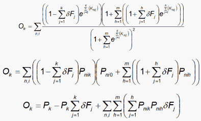
Then, since e^(x-δx) ≈ (1-δx)e^x for small δx,

Then ignoring cross-products of the δ terms and since δF₀ does not exist:

and similarly for the other categories, k=1,m.

At the end of each iteration, all the numerical values of the {O_k}, {P_k} and {ΣP_nikP_nih} terms are known. Consequently the {O_k} equations become a set of simultaneous linear equations which can be solved for {δF_j}. Then {F_j+δF_j} become the values of {F_j} for the next iteration after standardization so that Σ F_j = 0. So far, this estimation technique has proved robust and fast.

7. Multidimensionality and Singular-Value Decomposition (SVD).

Multidimensionality is a serious threat to the validity of unidimensional Rasch measures. It also degrades the capability of the measures to predict observations. Single-parameter fit statistics (such as INFIT, OUTFIT and point-biserial correlations) are insensitive to pervasive multidimensionality. PCA of residuals is a useful tool for investigating multidimensionality, but it loses its power as the proportion of missing data increases, and the number of variables to be factored increases. With 99% missing data and 17,770 variables, PCA of residuals is almost ineffective. It does signal the existence of secondary dimensions, but not in enough detail to be useful for item selection or improved prediction.

SVD is mathematical technique that has been used for decomposing matrices into a bilinear form for over 130 years. It is robust against missing data and the size of the matrix to be decomposed, so it is ideal for this application. SVD was the first conspicuously successful multi-dimensional method used by Netflix competitors. Most of those applied it using raw-score models.

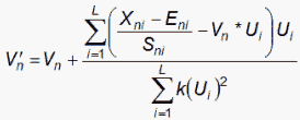
A first-level SVD model for the Netflix data, with SVD values {V_n} for the clients and {U_i} for the movies, is:

where

for the Andrich Rating-Scale model.

Notice that Rasch residuals are explained, as far as possible, by two factors (U for movies and V for clients) which multiply together. The factor products center on zero, because the residuals sum to zero.

Maximum-Likelihood Estimation: the starting values of {U_i} and {V_n} are random uniform numbers [-1,1] and normalization after each iteration through the data is Average(U_i²) = 1.

where k is chosen to prevent the iterative changes becoming too large.

There are now several options including:

A. The Rasch measures and the SVD values can be used to predict the Netflix Qualifying dataset. Further, a second-level SVD analysis can be performed on the residuals {ε_ni} from the first SVD analysis, and then the Qualifying dataset again predicted this time from two levels of SVD. This process can be continued for more SVD factors. During the Netflix competition, better prediction was achieved down to about 40 SVD factors.

B. From a Rasch data-analysis perspective, the first-level SVD conveniently segments the data into quarters: positive and negative SVD values for the movies, positive and negative SVD values for the clients. There is also a central core in which the movie and client SVD values are too small to be meaningful. They are ratings to which the first-level SVD "dimensions" do not apply. The 5 data subsets identified by the first-level SVD can then be used in 5 more Rasch analyses, and Rasch measures generated for further prediction. This process can also be continued.

We can also perform this computation for the standardized residuals:

where

which is the model S.D. of the observation around its expectation for the Andrich Rating-Scale model.

8. The Perils of Overfit When the Data Used for Estimation are also Predicted.

Netflix identified 1,408,395 ratings within the large Training dataset as the "Probe" dataset. They announced that the ratings in the Probe dataset had the same statistical characteristics as the ratings in the Quiz and Test datasets. Thus there were three similar datasets: the Probe dataset for which all the ratings were known, the Quiz dataset for which only the RMSRs for submissions were known, and the Test dataset about which nothing specific was known about the ratings. The Netflix Prize was awarded to the best prediction of the Test dataset.

The Probe dataset was only 1.4% of the Training dataset, but when it was included in the estimation process, the RMSR for the Probe data (predicted from the estimates) was noticeably lower than the RMSR reported for the Quiz data from the same set of measures. The inclusion of the data to be predicted within the estimation routine caused overfit to those data relative to the prediction of similar data not included in the estimation dataset.

Further, after each submission, an RMSR was obtained for the Quiz dataset. Over the months, this enabled a statistical picture of the Quiz dataset to be constructed which enabled some aspects of the prediction algorithms to be refined. The result was a slight overfit to the Quiz dataset. After the competition concluded, RMSRs for the Test dataset were released. The winner's RMSR on the Test dataset was 0.8567, but slightly better, 0.8554, on the somewhat more public Quiz dataset. The minimal extra information about the Quiz dataset was enough to produce slight overfit to the Quiz dataset relative to the completely unknown Test dataset.

We can speculate about what the winning RMSR would have been if competitors had only been given the Training dataset and the list of ratings to be predicted. In this "real life" situation, competitors would receive no feedback about the success of their submissions or the statistical properties of the ratings to be predicted until the competition concluded. My guess is that the best RMSR would have been close to 0.90 instead of 0.86.

9. Amazingly Low Variance-Explained.

Analysts are sometimes perturbed to see the low percentage of the variance in the observations explained by the Rasch measures. According to RMT 20:1, 1045, www.rasch.org/rmt/rmt201a.htm - the variance-explained by the Rasch measures is often 50% or less. But can other models do any better? The S.D. of the Test dataset around its mean is 1.1291. The winning RMSR is 0.8567, so the variance explained by the winning submission after 34 months work is (1.1291² - 0.8567²) / 1.1291² = 42%, less than 50%, despite using the most elaborate statistical procedures available. In fact, one month after the competition started, on Nov. 2, 2006, the best RMSR was around 0.9042, this was (1.1291² - 0.9042²)/1.1291² = 36% variance-explained. In the other 33 months of the competition, only 6% more variance was explained despite Herculean efforts by an army of computer scientists equipped with a huge amount of computing power, all expended in an effort to win the Netflix Prize of $1 million.

What does this mean in practice? The prize-winning RMSR was 0.8567. The mean-absolute-deviation is about 0.8*RMSR = 0.8*0.8567 ≈ 0.7. So, if prediction of exact Star ratings is needed, even the best set of predictions can be expected to be errant by 1 or more Stars more often than they are dead on.

John Michael Linacre

Linacre J.M. (2009) Rasch Lessons from the Netflix® Prize Challenge Competition, Rasch Measurement Transactions, 2009, 23:3, 1224-7

Rasch-Related Resources: Rasch Measurement YouTube Channel
Rasch Measurement Transactions & Rasch Measurement research papers - free	An Introduction to the Rasch Model with Examples in R (eRm, etc.), Debelak, Strobl, Zeigenfuse	Rasch Measurement Theory Analysis in R, Wind, Hua	Applying the Rasch Model in Social Sciences Using R, Lamprianou	El modelo métrico de Rasch: Fundamentación, implementación e interpretación de la medida en ciencias sociales (Spanish Edition), Manuel González-Montesinos M.
Rasch Models: Foundations, Recent Developments, and Applications, Fischer & Molenaar	Probabilistic Models for Some Intelligence and Attainment Tests, Georg Rasch	Rasch Models for Measurement, David Andrich	Constructing Measures, Mark Wilson	Best Test Design - free, Wright & Stone Rating Scale Analysis - free, Wright & Masters
Virtual Standard Setting: Setting Cut Scores, Charalambos Kollias	Diseño de Mejores Pruebas - free, Spanish Best Test Design	A Course in Rasch Measurement Theory, Andrich, Marais	Rasch Models in Health, Christensen, Kreiner, Mesba	Multivariate and Mixture Distribution Rasch Models, von Davier, Carstensen
Rasch Books and Publications: Winsteps and Facets
Applying the Rasch Model (Winsteps, Facets) 4th Ed., Bond, Yan, Heene	Advances in Rasch Analyses in the Human Sciences (Winsteps, Facets) 1st Ed., Boone, Staver	Advances in Applications of Rasch Measurement in Science Education, X. Liu & W. J. Boone	Rasch Analysis in the Human Sciences (Winsteps) Boone, Staver, Yale	Appliquer le modèle de Rasch: Défis et pistes de solution (Winsteps) E. Dionne, S. Béland
Introduction to Many-Facet Rasch Measurement (Facets), Thomas Eckes	Rasch Models for Solving Measurement Problems (Facets), George Engelhard, Jr. & Jue Wang	Statistical Analyses for Language Testers (Facets), Rita Green	Invariant Measurement with Raters and Rating Scales: Rasch Models for Rater-Mediated Assessments (Facets), George Engelhard, Jr. & Stefanie Wind	Aplicação do Modelo de Rasch (Português), de Bond, Trevor G., Fox, Christine M
Exploring Rating Scale Functioning for Survey Research (R, Facets), Stefanie Wind	Rasch Measurement: Applications, Khine	Winsteps Tutorials - free Facets Tutorials - free	Many-Facet Rasch Measurement (Facets) - free, J.M. Linacre	Fairness, Justice and Language Assessment (Winsteps, Facets), McNamara, Knoch, Fan

Forum

Rasch Measurement Forum to discuss any Rasch-related topic

Go to Top of Page
Go to index of all Rasch Measurement Transactions
AERA members: Join the Rasch Measurement SIG and receive the printed version of RMT
Some back issues of RMT are available as bound volumes
Subscribe to Journal of Applied Measurement

Go to Institute for Objective Measurement Home Page. The Rasch Measurement SIG (AERA) thanks the Institute for Objective Measurement for inviting the publication of Rasch Measurement Transactions on the Institute's website, www.rasch.org.

The URL of this page is www.rasch.org/rmt/rmt233d.htm

Website: www.rasch.org/rmt/contents.htm