Percentages with Continuous Rasch Models

In principle a continuous Rasch model is straightforward. The "ordinal" categories are the "dx" of differential calculus. The problem is that an arbitrary function must be imposed on the continuous data in order for the continuous model to be estimable. In my experimentation, Fourier transformations were the most successful functions.
Experiments with empirical data indicate that continuous data tend to have a granularity based on the way in which the observations are made, recorded, transmitted and their precision and their meaning. For instance, human heights may be recorded to the nearest inch and human weights to the nearest pound, though both height and weight are conceptually continuous.
Consequently, a useful approach is to examine the empirical data with a view to identifying the granularity. Count the granules as ordinal categories. Then standard ordinal Rasch models can be applied. The model ICC becomes the basis for deriving a continuous function, if that is required.

Percentages can be analyzed as continuous variables (like weight and time) or as discrete monotonic ratings (like Likert scales). Here, they are considered to be continuous. Percentages are expressed numerically. This implies that they are linear in form, and so can be manipulated arithmetically. But they are not usually linear in function, consequently arithmetical manipulation may not maintain their substantive implications.

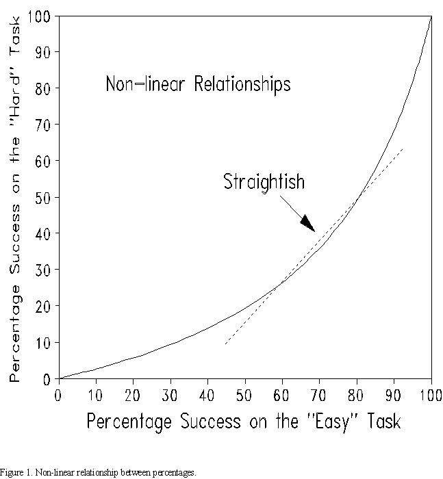
To illustrate, compare percentage success on the "Easy" test (or task) versus the "Hard" test. The test could be an achievement test in Math, or the test could be "households with electricity in the school district" versus "households with TVs". Figure 1 illustrates the inevitable relationship between the percentages.

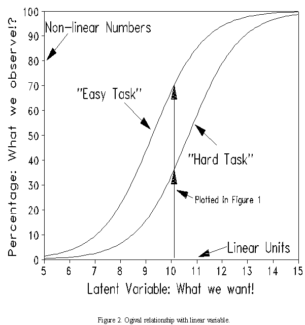
Both the "Easy" and "Hard" test are surrogates for, or indicators of, the latent variable which is the real focus of interest. This could be "math achievement" for the math tests. "Modernity" or "affluence" for the electricity/TV tests. Figure 2 shows the non-linear, ogival relationship between the percentage indicators and the desired latent variable.

The problem addressed by this paper is that of constructing sample-distribution-independent transformations of percentages onto the linear scale of the latent variable. For dichotomies and rating scales, the necessary and sufficient solution remains the familiar forms of the Rasch model.

A percentage scale, with the range 0% to 100%, reported with integers, has the form of a rating scale with 101 categories. This can be modeled directly as a polytomous Rasch scale with 100 step calibrations, i.e., 100 between-category transitions. In practice, however, many percentage values may not be observed. Further, the estimates of these 100 rating scale parameters tend to be based on thin data, and so are unstable across data sets. Also they are hard to interpret.

Modeling the percentage scale as approximating a continuous scale allows the choice of a measurement function with fewer parameters, more stability, and robustness against unobserved categories. Muller (1987) and Pedler (1987) derived restricted versions of a continuous Rasch model from Andrich's rating scale model formulations. A general form (Linacre, 1988), derived in Appendix A, is here applied to percentages in the range 0-100:

where P_nix = the probability density that person n will be observed, on item i, with value x, 0x100.

B_n, D_i, are the linear measures of person n and item i.

G(x) is a continuous function of k defining the percentage scale such that G(0) = 0 and G(100) = 0. The differential of G(x) is the step calibration at any point along the continuous rating scale.

The continuous function, G(x), is underdefined by the observed ratings and its form must be specified by the analyst. Since the aim of the measurement model is to assist in the interpretation and generalizability of measures, the optimum function, G(x), is one with a few, readily-interpretable, parameters. The success of the choice of function is indicated by the fit of the data to the model. Since this choice is made on prescriptive measurement criteria, rather those of descriptive statistics, it is the fit of the data to the model, rather than that of the model to the data that is paramount. This implies that an interpretable and generalizable model is to be preferred to a convoluted model with better statistical fit. Fortunately, experience with making similar choices for polytomous rating scale models indicates that the analyst has considerable latitude in the choice of functions. A wide choice of functions produces effectively equivalent numerical and substantive consequences.

Potentially productive functions are polynomials and trigonometric transformations. The functions become more immediately comprehensible when the range of the percentages is transformed from "0"-"100" to "0" to "+1" for polynomials, or "0" to "" for trigonometric functions.

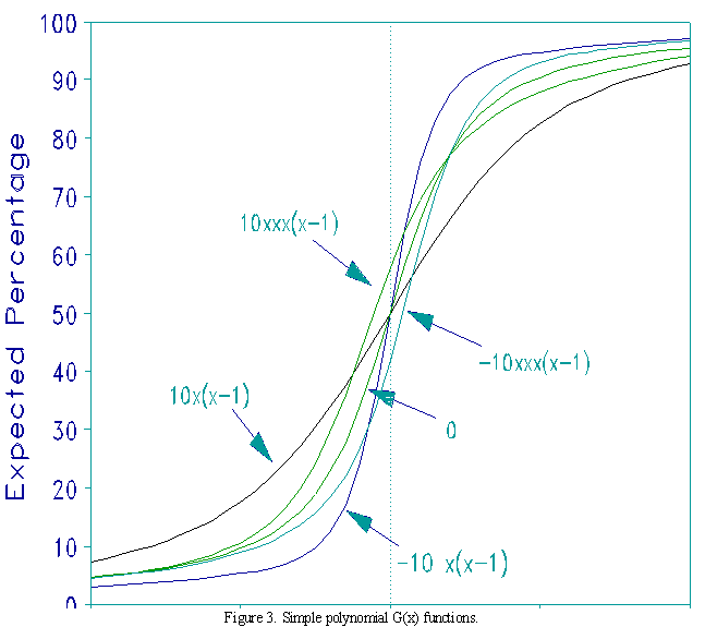
Figure 3 shows the impact on the item characteristic curve of various choices of simple polynomials. Functions G(x) = ax(x-1) and G(x) = ax³(x-1) both meet the condition G(0)=G(1)=0. The plots show the shapes produced by choosing a at -10, 10 and 0. It is seen that here, at least, the ICCs are relatively robust against changes in a and in function form.

Example: The Box shows percentages from Hartog and Rhodes (1935). For the function: G(x) = ax(x-1), the value a=-.46 is estimated with the estimation equations shown in Appendix B. This value is close to the central trace line in Figure 3.

                 Rater
Obj. 1  2  3  4  5  6  7  8  9 10 11 12 13
------------------------------------------
 1| 27 32 45 27 32 30 33 40 41 35 44 35 27
 2| 32 40 47 26 35 41 29 40 48 36 45 34 33
 3| 34 40 44 36 38 39 28 42 55 30 52 43 42
 4| 08 27 26 16 24 19 18 21 35 18 20 21 23
 5| 23 39 42 26 35 36 40 35 50 31 48 32 42
 6| 32 40 40 29 36 36 35 37 47 35 49 38 41
 7| 40 45 51 42 46 44 46 43 54 47 52 47 48
 8| 55 56 59 51 53 49 45 51 57 52 54 52 53
 9| 10 33 35 22 31 29 32 31 47 24 41 30 25
10| 35 40 43 45 41 39 29 38 50 32 42 34 38
11| 15 26 33 15 20 14 29 22 44 24 36 19 23
12| 43 40 53 46 40 44 33 47 55 41 47 41 38
13| 43 37 42 36 28 40 38 40 50 35 49 35 38
14| 07 27 31 13 19 22 23 26 43 10 35 23 23
15| 08 20 20 08 13 12 16 18 37 13 31 15 15
        from Hartog & Rhodes, 1935

Appendix A. Derivation of the Model

Consider the Rasch rating scale model (Andrich, 1978) for m+1 ordinal integer categories, 0,..,m given by

where

B_n = ability of person n

D_i = difficulty of item i

F_k = difficulty of being observed in category k of the rating scale relative to category k-1.

Then

Since the sum of all the probabilities of all m+1 possible categories must be 1,

so that multiplying through by the arbitrary non-zero value, exp(0(B_n-D_i)-F₀), then solving for Pni0,

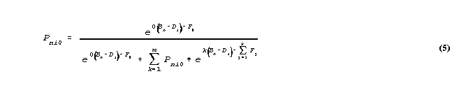
so that

For convenience, we define a cumulative difficulty function,

Note that the term G₀=F₀ is an arbitrary non-zero constant. It is conventionally set to 0.

Andersen (1977) points out that any equally-spaced scoring function produces estimates that have the properties of Rasch measures. Accordingly, rescore the 0,m category rating scale into m+1 ordinally counted categories from 0 to 1, each separated by the numerical interval 1/m. For convenience we will call this interval dx. Then such a scoring function meets the requirements of the Rasch model. The resulting measure estimates will be m times larger than those produced by the original unit scoring.

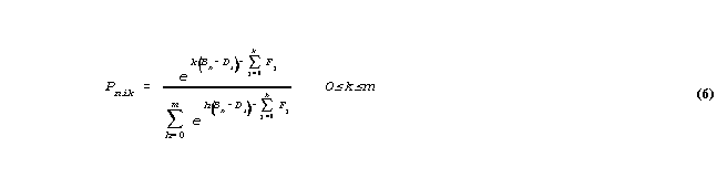
Let us consider the category x, for which we can now rewrite the equation 3 above as:

so that, making dx infinitesimal, so that the summations become integrations, and P_nix becomes the probability density function:

where

Here F(0)=G(0) is arbitrary, and, by convention, G(1)=0 for identifiability.

This is a general form of the continuous Rasch model, in which the form of the function G(x) is not specified. Particular forms of G(x) include polynomials, trigonometric and logarithmic functions.

Appendix B. Estimation Equations.

Simultaneous estimation of all parameters (JMLE) is preferred here because it is robust against missing data, and the statistical estimation bias is negligibly small due to the minimal likelihood of observing extreme scores in a relevant, non-trivial data set.

The estimation equations for the B_n and D_i are of the form (Wright and Masters, 1982):

where B_n is the current estimate and B'_n is the improved estimate. X_ni is the observation. E_ni is its expected value according to the model with the current parameter estimates. var(E_ni) is the model variance of the observation around its expectation.

In whatever way G(x) is defined, the following boundary conditions are imposed: G(0)=G(1)=0.

If G(x) = aH(x) + bJ(x), then the estimation equation for a is:

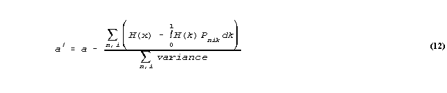
where a' is the improved estimate of a, and

We can apply this to particular functions, evaluated by numerical quadrature. For instance, if G(x) = ax(x-1), then G(0) = G(1) = 0, and

John Michael Linacre

Mueller, H. (1987). A Rasch model for continuous ratings. Psychometrika, 52, 165-181.

Pedler, P.J. (1987) Accounting for psychometric dependence with a class of latent trait models. Ph.D. dissertation. University of Western Australia.

This was an invited address to the SIG, AERA, 2000

Percentages with Continuous Rasch Models. Linacre, J.M. … Rasch Measurement Transactions, 2001, 14:4 p.771-4

Rasch Books and Publications
Invariant Measurement: Using Rasch Models in the Social, Behavioral, and Health Sciences, 2nd Edn. George Engelhard, Jr. & Jue Wang	Applying the Rasch Model (Winsteps, Facets) 4th Ed., Bond, Yan, Heene	Advances in Rasch Analyses in the Human Sciences (Winsteps, Facets) 1st Ed., Boone, Staver	Advances in Applications of Rasch Measurement in Science Education, X. Liu & W. J. Boone	Rasch Analysis in the Human Sciences (Winsteps) Boone, Staver, Yale
Introduction to Many-Facet Rasch Measurement (Facets), Thomas Eckes	Statistical Analyses for Language Testers (Facets), Rita Green	Invariant Measurement with Raters and Rating Scales: Rasch Models for Rater-Mediated Assessments (Facets), George Engelhard, Jr. & Stefanie Wind	Aplicação do Modelo de Rasch (Português), de Bond, Trevor G., Fox, Christine M	Appliquer le modèle de Rasch: Défis et pistes de solution (Winsteps) E. Dionne, S. Béland
Exploring Rating Scale Functioning for Survey Research (R, Facets), Stefanie Wind	Rasch Measurement: Applications, Khine	Winsteps Tutorials - free Facets Tutorials - free	Many-Facet Rasch Measurement (Facets) - free, J.M. Linacre	Fairness, Justice and Language Assessment (Winsteps, Facets), McNamara, Knoch, Fan
Other Rasch-Related Resources: Rasch Measurement YouTube Channel
Rasch Measurement Transactions & Rasch Measurement research papers - free	An Introduction to the Rasch Model with Examples in R (eRm, etc.), Debelak, Strobl, Zeigenfuse	Rasch Measurement Theory Analysis in R, Wind, Hua	Applying the Rasch Model in Social Sciences Using R, Lamprianou	El modelo métrico de Rasch: Fundamentación, implementación e interpretación de la medida en ciencias sociales (Spanish Edition), Manuel González-Montesinos M.
Rasch Models: Foundations, Recent Developments, and Applications, Fischer & Molenaar	Probabilistic Models for Some Intelligence and Attainment Tests, Georg Rasch	Rasch Models for Measurement, David Andrich	Constructing Measures, Mark Wilson	Best Test Design - free, Wright & Stone Rating Scale Analysis - free, Wright & Masters
Virtual Standard Setting: Setting Cut Scores, Charalambos Kollias	Diseño de Mejores Pruebas - free, Spanish Best Test Design	A Course in Rasch Measurement Theory, Andrich, Marais	Rasch Models in Health, Christensen, Kreiner, Mesba	Multivariate and Mixture Distribution Rasch Models, von Davier, Carstensen

Forum

Rasch Measurement Forum to discuss any Rasch-related topic

Go to Top of Page
Go to index of all Rasch Measurement Transactions
AERA members: Join the Rasch Measurement SIG and receive the printed version of RMT
Some back issues of RMT are available as bound volumes
Subscribe to Journal of Applied Measurement

Go to Institute for Objective Measurement Home Page. The Rasch Measurement SIG (AERA) thanks the Institute for Objective Measurement for inviting the publication of Rasch Measurement Transactions on the Institute's website, www.rasch.org.

The URL of this page is www.rasch.org/rmt/rmt144a.htm

Website: www.rasch.org/rmt/contents.htm