Paired Comparison: Measurement with Extreme Scores

Paired comparisons are a versatile and robust method for constructing measures: simple to collect, easy to analyze. There are drawbacks, however, particularly during the early stages of data collection.

An on-going analysis of the strength of NCAA basketball teams is underway. Since this analysis is intended to predict games not yet played, useful measures must be constructed from whatever data are available. Some teams do not experience their first win (or loss) until they have played six or more games. Finite measures are not estimable for these teams unless prior information is imposed on the measurement system. This brings a Bayesian element into the estimation procedure. Here are some implementations:

(a) Extreme Score Adjustment.

Only a discrete number of wins can be observed. We can suppose, however, that, an unbeaten team with W wins is manifesting the minimum ability for which that is the expected outcome. We can hypothesize that this is the ability corresponding to W - 0.33 wins and 0.33 losses. Any adjustment between 0.0 and 0.5 could be defended, but 0.33 has proved reasonable in other contexts (see RMT 12:2 632-3). Then the ability of the team is approximated by

where B_T is the ability of the team, M_T is the mean ability of the opposing teams and X_T is an expansion factor based on the dispersion of the opponents' abilities.

This correction has the counter-intuitive property that an unbeaten team is always estimated to be about 1 logit more able than a team playing a similar schedule, but with one loss. We would expect that, as the number of games played increased, the abilities of the two teams would approach equality.

(b) Imputed wins and losses.

We can implement the conviction that it is possible for all basketball teams to win on some occasions and to lose on other occasions. This can be done by imputing wins and losses against notional teams.

One approach is to posit a dummy team of ability corresponding to the mean ability of all observed teams. Against this dummy team, every team is awarded one extra win and one extra loss, whatever its win count W and loss count L. This central imputation produces a central bias in all measures, which decreases as the number of games played increases.

Another approach is to posit two dummy teams. One dummy team of such high ability that every observable team would likely lose against it. Another of such low ability that every team would win against it. Again, these wins and losses are awarded to all teams, and so bias all measures towards the center.

Through 11-30-98, a subset of 52 NCAA men's basketball teams had played against each other, producing wins and losses such that all measures were directly estimable in one frame of reference. A further 35 teams had played against these 52 teams, but had recorded only wins or losses against them. Thus there were 35 extreme scores. The number of games played between these 87 teams was 124.

By 12-22-98, these same 87 teams had played 203 games (64% more). Now all 87 had recorded both wins and losses against each other, so neither adjustment nor imputation was necessary. Which imputation method at 11-30 best predicts the 12-22 measures?

Extreme score correction only

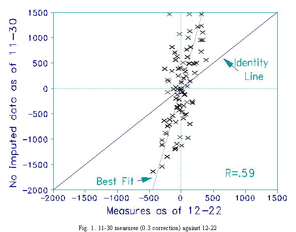
An adjustment of 0.3 score points is applied, but only to extreme scores. Fig. 1 shows that the measures for 11-30 have much greater dispersion than the reference measures for 12-22. The scaling is 100 units per logit. Since it is the relative measures of the teams that is the basis for inference, the local origins are set at 0 for convenience. Though the Pearson correlation between the measures is 0.59, their probabilistic meaning as paired comparisons is very different.

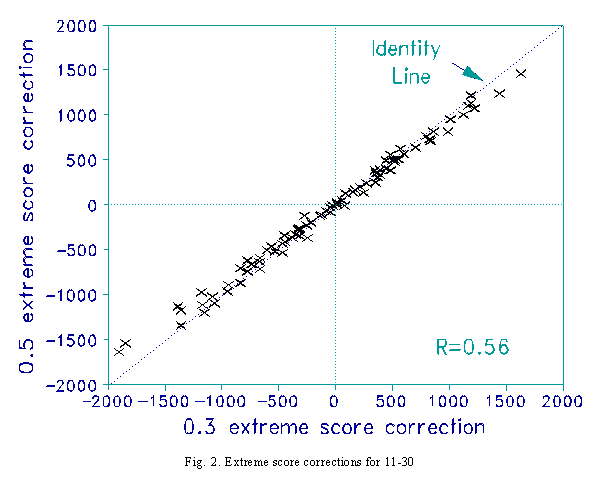
Increasing the extreme score adjustment to its maximum reasonable value of 0.5 has little effect. Fig. 2 shows that this slightly reduces the dispersion of extreme measures - but not enough to remove the effect seen in Fig. 1. Worse, the Pearson correlation with the 12-22 measures has degraded to 0.56.

Central imputation

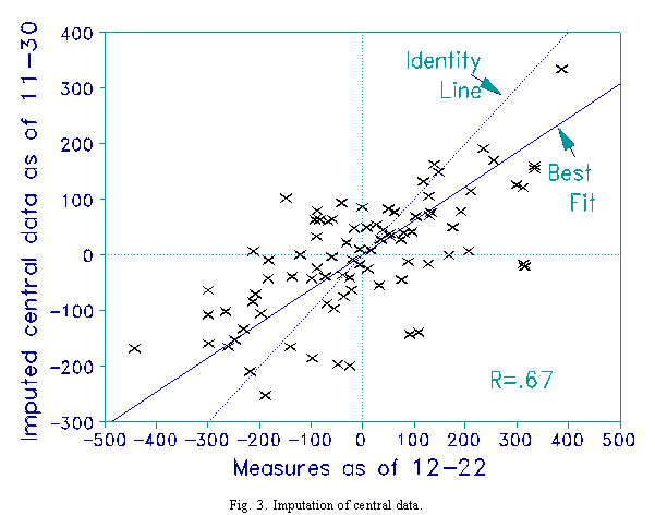
Each team is awarded one win and one loss against a notional team of average ability. But, in this example, each notional win or loss is assigned only half the weight of an observed game. Fig. 3 shows that the measures for 11-30 show less dispersion than those for 12-22. Even with the reduced weighting of imputed games, it can be seen that the measures crowd together in the center, reducing the prediction of winners to a toss-up. The Pearson correlation is 0.67.

Extreme imputation

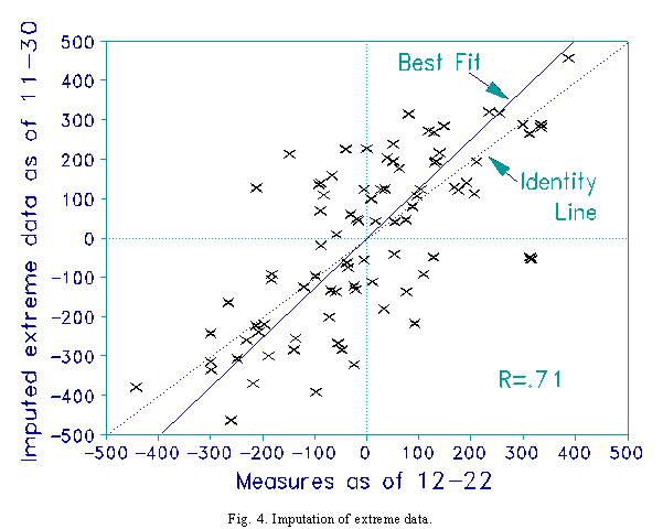
Each team is awarded a loss against a team 500 units (5 logits) above the mean, and a win against a team 500 units (5 logits) below the mean. These measures for the notional teams are in accord with the 12-22 measures, but were chosen based on pilot analyses using NCAA football data. Fig. 4 shows that the measures for 11-30 show slightly more dispersion than those for 12-22. The Pearson correlation is the highest yet, 0.71. It is this method of imputation that is the most successful with these data.

John M. Linacre

Paired comparison measurement with extreme scores.Linacre J.M. … Rasch Measurement Transactions, 1998, 12:3 p. 646-7.

Rasch-Related Resources: Rasch Measurement YouTube Channel
Rasch Measurement Transactions & Rasch Measurement research papers - free	An Introduction to the Rasch Model with Examples in R (eRm, etc.), Debelak, Strobl, Zeigenfuse	Rasch Measurement Theory Analysis in R, Wind, Hua	Applying the Rasch Model in Social Sciences Using R, Lamprianou	El modelo métrico de Rasch: Fundamentación, implementación e interpretación de la medida en ciencias sociales (Spanish Edition), Manuel González-Montesinos M.
Rasch Models: Foundations, Recent Developments, and Applications, Fischer & Molenaar	Probabilistic Models for Some Intelligence and Attainment Tests, Georg Rasch	Rasch Models for Measurement, David Andrich	Constructing Measures, Mark Wilson	Best Test Design - free, Wright & Stone Rating Scale Analysis - free, Wright & Masters
Virtual Standard Setting: Setting Cut Scores, Charalambos Kollias	Diseño de Mejores Pruebas - free, Spanish Best Test Design	A Course in Rasch Measurement Theory, Andrich, Marais	Rasch Models in Health, Christensen, Kreiner, Mesba	Multivariate and Mixture Distribution Rasch Models, von Davier, Carstensen
Rasch Books and Publications: Winsteps and Facets
Applying the Rasch Model (Winsteps, Facets) 4th Ed., Bond, Yan, Heene	Advances in Rasch Analyses in the Human Sciences (Winsteps, Facets) 1st Ed., Boone, Staver	Advances in Applications of Rasch Measurement in Science Education, X. Liu & W. J. Boone	Rasch Analysis in the Human Sciences (Winsteps) Boone, Staver, Yale	Appliquer le modèle de Rasch: Défis et pistes de solution (Winsteps) E. Dionne, S. Béland
Introduction to Many-Facet Rasch Measurement (Facets), Thomas Eckes	Rasch Models for Solving Measurement Problems (Facets), George Engelhard, Jr. & Jue Wang	Statistical Analyses for Language Testers (Facets), Rita Green	Invariant Measurement with Raters and Rating Scales: Rasch Models for Rater-Mediated Assessments (Facets), George Engelhard, Jr. & Stefanie Wind	Aplicação do Modelo de Rasch (Português), de Bond, Trevor G., Fox, Christine M
Exploring Rating Scale Functioning for Survey Research (R, Facets), Stefanie Wind	Rasch Measurement: Applications, Khine	Winsteps Tutorials - free Facets Tutorials - free	Many-Facet Rasch Measurement (Facets) - free, J.M. Linacre	Fairness, Justice and Language Assessment (Winsteps, Facets), McNamara, Knoch, Fan

Forum

Rasch Measurement Forum to discuss any Rasch-related topic

Go to Top of Page
Go to index of all Rasch Measurement Transactions
AERA members: Join the Rasch Measurement SIG and receive the printed version of RMT
Some back issues of RMT are available as bound volumes
Subscribe to Journal of Applied Measurement

Go to Institute for Objective Measurement Home Page. The Rasch Measurement SIG (AERA) thanks the Institute for Objective Measurement for inviting the publication of Rasch Measurement Transactions on the Institute's website, www.rasch.org.

The URL of this page is www.rasch.org/rmt/rmt1238.htm

Website: www.rasch.org/rmt/contents.htm