Extreme Raw Scores are Biased against Measures: Floor and Ceiling Effects

A new measurement in psychology has emerged from a confluence of scientific and social forces which are producing a revolution in social science methodology. We begin by reviewing how the semiotics of C.S.Peirce revise and enrich our interpretation of S.S. Stevens' four "kinds of measurement" into a creative dynamic for the evolution of one kind of useful measurement. Then we recall two turning points in social history which remind us of the antiquity and moral force of our need for stable measures. Next we review the psychometric and mathematical histories of measurement, show how the obstacles to inference shape our measurement practice and summarize Georg Rasch's contributions. This brings us to some applications of the "new" measurement models produced by Rasch's work. Finally we review some mistakes that the history of measurement can teach us to stop making.
Peirce Semiotics
Semiotics is the science of signs. It provides a developmental map of creative thought which shows how thinking progresses step-by-step from qualitative flashes of insight to the reproducible quantitative laws of process which are the tool and triumph of science. Table 1 outlines six levels of conscious signs through which science is reached (Buchler 1940, Sheriff 1994).
| C.S.Peirce 1903 |
Stevens 1939 |
W.Kinston 1985 |
6 STEPS TO SCIENCE |
| 5. possible ICON |
FANCY qualitative | ||
| 6. possible INDEX |
Entity real idea |
THOUGHT qualitative | |
| 7. factual INDEX |
Nominal | Observable existent |
OBJECT qualitative |
| 8. possible SYMBOL |
Ordinal | Comparable quantity |
SCORE quantitative |
| 9. factual SYMBOL |
Interval Ratio |
Measurable unit |
MEASURE quantitative |
| 10. arguable SYMBOL |
Relatable process |
RELATION quantitative | |
| Peirce's complete set of signs mark out ten steps in the evolution of knowing (Sheriff 1994). The four earliest steps, however, precede the kind of awareness we ordinarily recognize as scientific so they are omitted here. Note how Peirce improves on Stevens in two ways: 1) Twice as many identifiable steps. 2) A clear sequence of connected thinking from the wildest qualitative hypothesis to the most objectively quantitatively measured process. | |||
The first level of "scientific" consciousness is private "fancy", a flash of thought, a wild hypothesis. The thought is ours alone. We may never rethink it. Peirce calls this first level of awareness a "possible icon". It is the seed of creativity.
Then some wild ideas acquire meaning. We think them again and encounter others who also think them. This is the step to Peirce's second level. A particular idea becomes more than a private fancy. It becomes something to return to, to talk about. It is still but a quality. We cannot point and say, "There it is." But we can think and talk it. Eddington (1946) and Kinston (1985) call this level an "entity". Peirce calls it a "possible index".
The next step up is an invention of a way to "see" what we mean. We nominate an "experience", a "thing", to serve as an instance of our "idea". This makes our idea observable and "real". Now our idea is a thing of the world. We can do more than think it. We can seek it. We can count it. We have reached the third level at which Stevens'(1946) first "kind of measurement", the "nominal", finally emerges. Eddington and Kinston call this level an "observable" and Peirce calls it a "factual index".
Stevens Revised
Peirce's first two steps to science precede Stevens' "nominal". This shows us that a nominal is not where science begins. A nominal is only reached as a consequence of an evolution of prior possible icons and indices. It is the successful development of these precursors which bequeath the nominal its potential merit as a qualitative thought with quantitative possibilities. We dream before we think. We think before we point. The scientific harvest which may follow depends on the fertility of our imagination and the cultivation of our thought.
Then, as we gather examples of our evolving entity, we discover preference. Some "things" please us. Others do not. The presence and absence of our entities acquire irresistible valence. We begin to count on more of their "goodness", less of their "badness". Our preferences propel us to a fourth level, a higher sign, a "comparable", corresponding to Steven's "ordinal" kind of measurement. We discover that entity nomination is not only a necessary step toward science, but that we are unable to nominate without preferring. Steven's calls this "ordinal measurement". Peirce calls it a "possible symbol". Our choices and pursuits of this latency are the crucible in which the tools of science are forged.
At this stage the subtle and decisive invention of abstract quantification begins to emerge. Valuing more or less of particular "things" begins to imply valuing more or less of a common "something" these "things" imply, a latent variable. We begin to abstract from counting apples to ideas of "appleness".
To count is to begin to measure. But counting concrete objects is ambiguous. Counts of real objects do not maintain the magnitude equivalence necessary to qualify as measures. When bricks do not approximate a single size, each piece requires individual attention, building is hard to plan, requires continuous readjustment and suffers awkward irregularity. It takes uniform bricks to regularize construction, to draw plans. It is the same in trade. How could my grocer sell me a mix of apples and oranges without the currency they share.
This earthy necessity propels us upward to a fifth level. We invent an even more abstract sign, the Eddington and Kinston "measurable", which reaches beyond a comparison of "more" or "less" to build an imaginary variable along which we can define and maintain an ideal of perfectly equal units which, while abstract in theory, are, nevertheless, approximable in practice. Stevens calls this "interval measurement". Peirce calls it a "factual symbol". It is the fundamental language of science. We will discover that its successful realization requires clear ideas as to the obstacles to inference and an understanding of their mathematical solutions.
Stevens distinguishes ratios from intervals. But logarithms of ratios are intervals. And exponentiated intervals are ratios. If we have one, we have the other. The only basis for a distinction would be a belief in "natural origins". But there are none. Look around. We put our origins wherever they work best: either end of a yardstick, where water (or alcohol) becomes solid, where molecular motion is extrapolated to cease or.... Our origins are convenient reference points for useful theories. When our theories change so do our origins. (Wright & Masters 1982 p.9)
Stevens' taxonomy stops here. Peirce and Kinston reach one step further to the level of Peirce's "arguable symbol" and Kinston's "relatable". This is where theories of process begin. What good is one variable, if it does not lead to another? And no, at last, a job for linear statistics emerges. To see what our variables imply about process, we plot them against one another. We analyze their variance, estimate regressions and model equations.
Implications for Practice
Peirce's semiotics specify six steps which we must climb through to reach our pride of science. A quick regression of raw data is always misleading. When we do not think and build our way through the five steps which precede statistical analysis with care and meaning, our "research" comes up empty. We can always get some "numbers". But they will not add up to reproducible meaning.
Mistaking Stevens' nominal/ordinal/interval/ratio taxonomy as four "kinds of measurement", each with its own "kind of statistics", has polarized social scientists into a qualitative/quantitative antipathy which cuts off communication, paralyses progress and overlooks the inevitability of a careful stepwise evolution beginning two steps before Stevens' nominal and going a step beyond his interval/ratio to reach, not two or four kinds of measurement but just one kind of science.
The moment we nominate a possible index as sufficiently interesting to observe, we experience a preference which elevates that nominal to an ordinal. Then as we replicate our observations we cannot resist counting them and using these counts as though they were measures. The final step from concrete ordinals to abstract intervals is forced upon us by the necessities of commerce. Just as we cannot trade without currency, we cannot reason quantitatively without linear measures.
Thus the discovery, invention and construction of scientific knowledge begins with 1) a wild hypothesis which gets thought into 2) a reproducible idea, which becomes realized in 3) an observable instance, to be interpreted as 4) a concrete ordinal which is carefully built into 5) an abstract measurable suitable, finally, for analyses in relation to other measurables and so to the construction of 6) promising theories.
Long before science or mathematics emerged as professions the commercial, architectural, political and moral necessities for abstract, exchangeable units of unchanging value were recognized and pursued. A fair weight of seven was a tenant of faith among seventh century Muslims. Muslim leaders were censured for using less "righteous" standards. (Sears, 1997)
Twelve centuries ago Caliph 'Umar b. 'Abd al-'Aziz, ruled that:
The people of al-Kufa have been struck with trial, hardship, oppressive governments and wicked practices. The righteous law is justice and good conduct. I order you to take in taxes only the weight of seven. (Damascus, 723)
Seven centuries ago King John decreed that:
There shall be one measure of wine throughout Our kingdom, and one of ale, and one measure of corn, to wit, the London quarter, and one breadth of cloth, to wit, two ells within the selvages. As with measures so shall it be with weights. (Magna Carta, Runnymede, 1215)
Some say the crux of the French Revolution was outrage against unfair measures. The true origins of stable units for length, area, volume and weight were the necessities of commerce and politics. The steam engine is responsible for our measures of temperature and pressure.
Counting Events does NOT Produce Equal Units
The patriarch of educational measurement, Edward Thorndike, observed:
If one attempts to measure even so simple a thing as spelling, one is hampered by the fact that there exist no units in which to measure. One may arbitrarily make up a list of words and observe ability by the number spelled correctly. But if one examines such a list one is struck by the inequality of the units. All results based on the equality of any one word with any other are necessarily inaccurate. (Thorndike 1904, p.7)
Thorndike saw the irregularity in counting concrete events, however indicative they might seem (Engelhard 1991, 1994). One might observe signs of spelling. But simply counting would not measure spelling. The problem of entity ambiguity is ubiquitous in science, commerce and cooking. What is an apple? How many apples make a pie? How many little apples equal one big one? Why don't three apples always cost the same? With apples, we solve entity ambiguity by renouncing the concrete apple count and turning, instead, to abstract apple volume or weight. (Wright 1992, 1994)
Raw Scores are NOT Measures
Thorndike was not only aware of the "inequality of the units" counted but also of the non-linearity of the "raw scores" counting produced. Raw scores are bound to begin at "none right" and end at "all right". But the linear measures we intend raw scores to imply have no boundaries. Figure 1 is a typical raw score to measure ogive. It shows how the monotonically increasing ogival exchange of one more right answer for a measure increment is steepest in the middle where items are dense and flat at the extremes of 0% and 100%. One more right answer implies the least measure increment near 50%, but an infinite increment at each extreme. In Figure 1 the measure distance along the horizontal axis which corresponds to a 10 percentile raw score increment from 88% to 98% up the vertical axis is 5 times greater than the measure distance corresponding to a 10 percentile raw score increment from 45% to 55%.
| Number of Items |
Normal Test |
Uniform Test |
| 10 | 2.0 | 3.5 |
| 25 | 4.6 | 4.5 |
| 50 | 8.9 | 6.0 |
| 100 | 17.6 | 8.0 |
| These calculations are explained on pages
143-151 of Best Test Design (Wright & Stone
1979). The ratio for a normal test of L
items is: loge{2(L-1)/(L-2)}/loge{(L+2)/(L-2)} | ||
Table 2 shows the numerical magnitude of this raw score bias against extreme measures for tests of normally distributed and uniformly distributed item difficulties. The tabled values are ratios formed by dividing the measure increment corresponding to one more right answer at the next to largest extreme step by the measure increment corresponding to one more right answer at the smallest central step. Even when item difficulties spread out uniformly in equal increments, the raw score bias against measure increments at the extremes of a 25 item test is a factor of 4.5. When the item difficulties of a 50 item test distribute normally, the bias against extreme measures is a factor of 8.9!
Raw score bias is not confined to dichotomous responses. The bias is just as severe for partial credits, rating scales and, of course, the infamous Likert Scale, the misuse of which pushed Thurstone's seminal 1920's work on how to construct linear measures from ordinal raw scores out of use.
This raw score bias in favor of central scores and against extreme scores means that any linear statistical method like analysis of variance, regression, generalizability, LISREL or factor analysis that misuses non-linear raw scores or Likert scales as though they were linear measures will produce systematically distorted results. Like the non-linear raw scores on which they are based, all results will be target biased and sample dependent and hence inferentially ambiguous. (Wright & Stone 1979 pp 4-9, Wright & Masters 1982 pp 27-37, Wright & Linacre 1989) Little wonder that so much social "science" remains transient description of never to be reencountered situations, easy to doubt with almost any replication.
An obvious first law of measurement is:
Before applying linear statistical methods, use a measurement model to construct linear measures from your observed raw data.
There are many advantages to working with model-controlled linearization. Each measure is accompanied by a realistic estimate of its precision and a mean square residual-from-expectation evaluation of the extent to which the raw ordinal data from which the measure has been estimated fit the measurement model. When we now advance to graphing results and applying linear statistics to analyze relationships among variables, we not only have linear measures to work with, we also have estimates of their statistical precision and validity.
Thurstone's Measurement
Between 1925 and 1932 Louis Thurstone published 24 articles and a book on how to construct good measures.
Unidimensionality:
The measurement of any object or entity describes only one attribute of the object measured. This is a universal characteristic of all measurement. (Thurstone 1931, p.257)
Linearity:
The very idea of measurement implies a linear continuum of some sort such as length, price, volume, weight, age. When the idea of measurement is applied to scholastic achievement, for example, it is necessary to force the qualitative variations into a scholastic linear scale of some kind. (Thurstone & Chave 1929, p.11)
Abstraction:
The linear continuum which is implied in all measurement is always an abstraction...There is a popular fallacy that a unit of measurement is a thing - such as a piece of yardstick. This is not so. A unit of measurement is always a process of some kind...
Invariance:
... which can be repeated without modification in the different parts of the measurement continuum. (Thurstone 1931, p.257)
Sample-free item calibration:
The scale must transcend the group measured. One crucial test must be applied to our method of measuring attitudes before it can be accepted as valid. A measuring instrument must not be seriously affected in its measuring function by the object of measurement...Within the range of objects...intended, its function must be independent of the object of measurement. (Thurstone 1928, p.547)
Test-free person measurement:
It should be possible to omit several test questions at different levels of the scale without affecting the individual score ... It should not be required to submit every subject to the whole range of the scale. The starting point and the terminal point...should not directly affect the individual score. (Thurstone 1926, p.446)
Guttman's Scale
In 1944 Louis Guttman showed that the meaning of a raw score, including one produced by Likert scales, would be ambiguous unless the score defined a unique response pattern.
If a person endorses a more extreme statement, he should endorse all less extreme statements if the statements are to considered a scale...We shall call a set of items of common content a scale if [and only if] a person with a higher rank than another person is just as high or higher on every item than the other person. (Guttman 1950, p.62)
According to Guttman only data which approximate this kind of conjoint transitivity can produce unambiguous measures. A deterministic application of Guttman's "scale" is impossible. But his ideal of conjoint transitivity is the kernel of Norman Campbell's (1920) fundamental measurement. Notice the affinity between Guttman's "scalability" and Ronald Fisher's "sufficiency" (Fisher 1922). Both call for a statistic which exhausts the information to which it refers.
Although mathematics did not initiate the practice of measurement, it is the mathematics of measurement which provide the ultimate foundation for better practice and the final logic by which useful measurement evolves and thrives. As we review some of the ideas by which mathematicians and physicists built their theories, we will discover that, although each worked on his own ideas in his own way, their conclusions converge to a single formulation for measurement practice.
Concatenation
In 1920 physicist Norman Campbell deduced that the "fundamental" measurement on which physics was built required the possibility of explicit concatenation, like joining the ends of sticks to concatenate length or piling bricks to concatenate weight. Because psychological concatenation seemed impossible, Campbell concluded that there could be no fundamental measures in psychology.
Sufficiency
In 1920 Ronald Fisher, while applying his "likelihood" version of inverse probability to invent maximum likelihood estimation, discovered a statistic so "sufficient" that it exhausted from the data in hand all information concerning its modeled parameter. Fisher's discovery is much appreciated for its informational efficiency. But it has a concomitant property which is far more important to the construction of measurement. A statistic which exhausts all modelled information enables conditional formulations by which a value for each parameter can be estimated independently of the values of all other parameters in the model.
This follows because the functional presence of any parameter can be replaced by its sufficient statistic (Andersen 1977). Without this replacement each parameter estimation, each attempt to construct a generalizable measure, is forever foiled. The incidental distributions of the other parameters make every "measure" estimate situation-specific. Generality is destroyed.
This leads to a second law of measurement:
When a model employs parameters for which there are no sufficient statistics, that model cannot construct useful measurement because it cannot estimate its parameters independently of one another.
Divisibility
In 1924 Paul Levy (1937) proved that the construction of a law for probability distributions which is "stable" with respect to arbitrary decisions as to what is countable required infinitely divisible parameters (Feller 1950, 271). Levy's divisibility is logarithmically equivalent to conjoint additivity (Luce & Tukey 1964). Levy's conclusions were reenforced in 1932 when A.N.Kolmogorov (1950 pp.9 & 57) proved that independent parameter estimation also requires divisibility.
In 1992 Abe Bookstein reported his astonishment at the mathematical equivalence of every counting law he could find (1992, 1996). Provoked to decipher how this ubiquitous equivalence could have occurred, he discovered that the counting formulations were not only members of one simple mathematical family, but that they were surprisingly robust with respect to ambiguities of entity (which elements to count), aggregation (at what hierarchical level to count) and scope (for how long and how far to count). As he sought to understand the source of this remarkable robustness Bookstein discovered that the necessary and sufficient formulation was Levy's divisibility.
Additivity
American work on the mathematical foundations of measurement came to fruition with the proof by Duncan Luce and John Tukey (1964) that Campbell's concatenation was a physical realization of the mathematical law which is necessary for fundamental measurement.
The essential character of simultaneous conjoint measurement is described by an axiomatization for the comparison of effects of pairs formed from two specified kinds of "quantities"... Measurement on interval scales which have a common unit follows from these axioms.
A close relation exists between conjoint measurement and the establishment of response measures in a two-way table ...for which the "effects of columns" and the "effects of rows" are additive. Indeed the discovery of such measures...may be viewed as the discovery, via conjoint measurement, of fundamental measures of the row and column variables. (Luce & Tukey 1964, p.1)
Their conclusion writes a third law of measurement:
When no natural concatenation operation exists, one should try to discover a way to measure factors and responses such the "effects" of different factors are additive. (Luce & Tukey 1964, p.4)
The common measures by which we make life better are so familiar that we seldom think about "why" or "how" they work. A mathematical history of inference, however, takes us behind practice to the theoretical requirements which make measurement possible. Table 3 articulates an anatomy of inference into four obstacles which stand between raw data and the stable inference of measures they might imply.
| OBSTACLES | SOLUTIONS | INVENTORS |
| UNCERTAINTY have -> want now -> later statistic -> parameter |
PROBABILITY binomial odds regular irregularity misfit detection |
Bernoulli 1713 Bayes 1764 Laplace 1774 Poisson 1837 |
| DISTORTION non-linearity unequal intervals incommensurability |
ADDITIVITY linearity concatenation conjoint additivity |
Fechner 1860 Helmholtz 1887 N.Campbell 1920 Luce/Tukey 1964 |
| CONFUSION interdependence interaction confounding |
SEPARABILITY sufficiency invariance conjoint order |
Rasch 1958 R.A.Fisher 1920 Thurstone 1925 Guttman 1944 |
| AMBIGUITY of entity, interval and aggregation |
DIVISIBILITY independence stability reproducibility exchangeability |
Levy 1924 Kolmogorov 1932 Bookstein 1992 de Finetti 1931 |
Uncertainty is our motivation for inference. The future is uncertain by definition. We have only the past by which to foresee. Our solution is to capture this uncertainty in a matrix of inverse probabilities which regularize the irregularities that interrupt the continuity between what seems certain now but must be uncertain later.
Distortion interferes with the transition from observation to conceptualization. Our ability to figure things out comes from our faculty to visualize. Our power of visualization evolves from the survival value of body navigation through the space in which we live. Our antidote to distortion is to represent our observations of experience in the bi-linear form that makes them look like the mostly two dimensional space we see in front of us. To "see" what experience "means", we "map" it.
Confusion is caused by interdependencies. As we look for tomorrow's probabilities in yesterday's lessons, confusing interactions intrude. Our resolution of confusion is to simplify the complexity we experience into a few shrewdly crafted "dimensions". We define and measure our dimensions one at a time. Their authority is their utility. "Truths" may be unknowable. But when our inventions "work", we have proven them "useful". And when they continue to work, we come to believe in them and may even christen them "real" and "true".
Ambiguity, a fourth obstacle to inference, occurs because there is no objective way to determine exactly which operational definitions of conceptual entities are the "right" ones. As a result only models which are indifferent to level of composition are robust enough to survive the vicissitudes of entity ambiguity. Bookstein (1992) shows that this requires functions which embody divisibility or additivity as in:
Fortunately the mathematical solutions to Distortion, Confusion and Ambiguity are identical. The parameters that govern the probability of the data must appear in either an entirely divisible or an entirely additive form. No mixtures of divisions and additions, however, are admissible.
The Probability Solution
The application of Jacob Bernoulli's 1713 binomial distribution as an inverse probability for interpreting the implications of observed events (Thomas Bayes, 1764, Pierre Laplace, 1774 in Stigler 1986, pp. 63-67, 99-105) was a turning point in the mathematical history of measurement. Our interests reach beyond the data in hand to what these data might imply about future data, still unmet, but urgent to foresee.
The first problem of inference is how to predict values for these future data, which, by the meaning of "inference", are necessarily "missing". This meaning of "missing", of course, must include not only the future data to be inferred but also all possible past data which were lost or never collected. Since the purpose of inference is to estimate what future data might be like before they occur, methods which require complete data (i.e. cannot analyze present data in which some values are missing) cannot be methods of inference. This realization engenders a fourth law of measurement:
Any statistical method nominated to serve inference which requires complete data, by this requirement, disqualifies itself as an inferential method.
But, if what we want to know is "missing", how can we use the data in hand to make useful inferences about the "missing" data they might imply? Inverse probability reconceives our raw observations as a probable consequence of a relevant stochastic process with a useful formulation. The apparent determinism of formulae like F = MA depends on the prior construction of relatively precise measures of F and M (For a stochastic discussion of this formulation of the "multiplicative law of accelerations" in which M is realized by solid bodies and F is realized by instruments of force, see Rasch 1960, 110-114). The first step from raw observation to inference is to identify the stochastic process by which an inverse probability can be defined. Bernoulli's binomial distribution is the simplest process. The compound Poisson is the stochastic parent of all such measuring distributions (Rasch 1960, 122).
The Mathematical Solution
The second problem of inference is to discover which mathematical models can determine the stochastic process in a way that enables a stable, ambiguity resilient estimation of the model's parameters from data in hand. At first glance, this step may look obscure. Table 3 suggests that its history followed many paths, traveled by many mathematicians and physicists. One might fear that there was no clear second step but only a variety of unconnected possibilities with seemingly different resolutions. Fortunately, reflection on the motivations for these paths and examination of their mathematics leads to a reassuring simplification. Although each path was motivated by a particular concern as to what inference must overcome to succeed, all solutions end up with the same simple, easy to understand and easy to use formulation. The mathematical function which governs the inferential stochastic process must specify parameters which are either infinitely divisible or conjointly additive i.e. separable.
What does this summarize to?
1. Measures are inferences,
2. Obtained by stochastic approximations,
3. Of one dimensional quantities,
4. Counted in abstract units,
5. Which are impervious to extraneous factors.
To meet these requirements,
Measurement must be an inference of values for infinitely divisible parameters which define the transition odds between observable increments of a theoretical variable.
The Fundamental Measurement Model
In 1953 Georg Rasch (1960) found that the only way he could compare performances on different tests of oral reading was to apply the exponential additivity of Poisson's 1837 distribution (Stigler 1986, pp.182-183) to data produced by a sample of students responding simultaneously to both tests. Rasch used the Poisson distribution as his model because it was the only distribution he could think of that enabled the equation of two tests to be entirely independent of the obviously arbitrary distribution of the reading abilities of the sample.
As Rasch worked out his solution to what became an unexpectedly successful test equating, he discovered that the mathematics of the probability process, the measurement model, must be restricted to formulations which produced sufficient statistics. Only when his parameters had sufficient statistics could these statistics replace and hence remove the unwanted person parameters from his estimation equations and so obtain estimates of his test parameters which were independent of the incidental values of the person parameters used in the model.
I never heard Rasch refer to Guttman's conjoint transitivity. Yet, as Rasch describes the necessities of his probability function, he defines a stochastic solution to the impossible requirement that data conform to a deterministic conjoint transitivity.
A person having a greater ability than another should have the greater probability of solving any item of the type in question, and similarly, one item being more difficult than another one means that for any person the probability of solving the second item correctly is the greater one. (Rasch 1960, p.117)
Rasch completes his argument for a measurement model on pages 117-122 of his 1960 book. His "measuring function" on page 118 specifies the divisible definition of fundamental measurement for dichotomous observations as:
where P is the probability of a correct solution, f(P) is a function of P, still to be determined, b is a ratio measure of person ability and d is a ratio calibration of item difficulty.
Rasch explains this "measuring function" as an inverse probability "of a correct solution, which may be taken as the imagined outcome of an indefinitely long series of trials (p.118). Because "an additive system...is simpler than the original...multiplicative system," Rasch takes logarithms:
and transforms P into its logistic form:
Then Rasch asks: "Does there exist a function of the variable L which forms an additive system in parameters for person B and parameters for items D such that:
(pp.119-120)
Finally, asking "whether the measuring function for a test, if it exists at all, is uniquely determined" Rasch proves that:
"is a measuring function for any positive values of C and A, if f0(P) is", which "contains all the possible measuring functions which can be constructed from f0(P). So that "By suitable choice of dimensions and units, i.e. of A and C for f(P), it is possible to make the b's and d's vary within any positive interval which may...be...convenient" (p.121).
Because of "the validity of a separability theorem (due to sufficiency):
It is possible to arrange the observational situation in such a way that from the responses of a number of persons to the set of items in question we may derive two sets of quantities, the distributions of which depend only on the item parameters, and only on the personal parameters, respectively. Furthermore the conditional distribution of the whole set of data for given values of the two sets of quantities does not depend on any of the parameters (p.122).
With respect to separability the choice of this model has been lucky. Had we for instance assumed the "Normal-Ogive Model" [as did Thurstone in the 1920's] with all si = 1 - which numerically may be hard to distinguish from the logistic - then the separability theorem would have broken down. And the same would, in fact, happen for any other conformity model which is not equivalent - in the sense of f(P) = C{f0(P)}A to f(P) = b/d...as regards separability.
The possible distributions are...limited to rather simple types, but...lead to rather far reaching generalizations of the Poisson...process (p.122).
The Compound Poisson
Rasch (1960, 1961, 1963, 1968, 1969, 1977) shows that formulations in the compound Poisson family, such as Bernoulli's binomial, are not only sufficient for the construction of stable measurement, but that the "multiplicative Poisson" (Feller 1957, 270-271) is the only mathematical solution to the formulation of an objective, sample and test-free measuring function. Andrich (1995, 1996) confirms that Rasch separability requires the Poisson distribution for estimating measures from discrete observations. Bookstein (1996) shows that the stochastic application of the divisibility necessary for ambiguity resilience requires the compound Poisson.
Conjoint Additivity and Rasch
Although conjoint additivity is acknowledged to be a decisive theoretical requirement for measurement, few psychologists realize that Rasch models are its practical realization. Rasch models construct conjoint additivity by applying inverse probability to empirical data and then testing these data for their goodness-of-fit to this construction (Keats 1967, Fischer 1968, Perline, Wright, Wainer 1978).
The Rasch model is a special case of additive conjoint measurement... a fit of the Rasch model implies that the cancellation axiom (i.e. conjoint transitivity) will be satisfied...It then follows that items and persons are measured on an interval scale with a common unit. (Brogden 1977, p.633)
Rasch models are the only laws of quantification which define objective measurement, determine what is measurable, decide which data are useful and expose which data are not.
Our data can be obtained as responses to nominal categories like:
yes/no
right/wrong
present/absent
always/usually/sometimes/never
strongly agree/agree/disagree/strongly disagree
Nominal labels like these invite ordinal interpretation from more to less: more yesness, more rightness, more presence, more occurrence, more agreement. Almost without further thought, we take the asserted hierarchy for granted and imagine that our declared categories will inevitably implement a clear and stable ordinal scale. But whether our respondents actually use our categories in the ordered steps we intend cannot be left to imagination. We must find out by analyzing actual responses how respondents actually use our categories. When this is carefully done, it frequently emerges that an intended rating scale of five or six seemingly ordinal categories has actually functioned as a simple dichotomy.
Binomial transition odds like Pnix/Pnix-1 can implement the inferential possibilities of data collected in nominal categories interpreted as ordered steps. When we label our categories: x = 0,1,2,3,4,,, in their intended order, then each numerical label can count one more step up our ordered scale.
| WRONG x = 0 |
RIGHT x = 1 |
| STRONGLY DISAGREE x = 0 |
DISAGREE x = 1 |
AGREE x = 2 |
STRONGLY AGREE x = 3 |
We can connect each x to the situation for which we are trying to construct measures by subscribing x as xni so that it can stand for a rating recorded by (or for) a person n on an item i and then specify Pnix as the inverse probability that person n obtains x as their rating on item i.
The transition odds that the rating is x rather than x - 1 become Pnix/Pnix-1.
| Pnix-1 | Pnix | ||
| x - 2 | x - 1 | x | x + 1 |
Then we can introduce a mathematical model which "explains" Pnix as the consequence of a conjointly additive function which specifies exactly how we want our parameters to govern Pnix.
Our parameters can be Bn, the location measure of person n on the continuum of reference; Di, the location calibration of item i, the instrumental operationalization of this continuum and Fx, the gradient up the continuum of the transition from response category (x-1) to category (x).
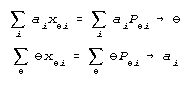
The necessary and sufficient measurement models are:
in which the symbol "==" means "by definition" rather than merely "equals".
The first model satisfies the Levy/Kolmogorov/Bookstein divisibility requirement. The second model satisfies the Campbell/Luce/Tukey conjoint additivity requirement. On the left of either formula a concrete datum xni is replaced by its abstract Bernoulli/Bayes/Laplace stochastic proxy Pnix.
In practice we apply the second formulation because its additivity produces parameter estimates in the linear form to which our eyes and feet are so accustomed. Our penchant for linearity is more than visual. Fechner (1860) showed that when we experience a ratio impact of light, sound or pain, our nervous system takes a logarithm so that we can see how the impact feels on a linear scale. Nor was Fechner the first to notice this neurology. Pythagorean tuning puts musical instruments out of tune at each key change. Tuning to notes which increase in frequency by equal ratios, however, produces an "equally tempered" scale of notes which sound equally spaced in any key. Pythagorean tuning is key-dependent. Equally tempered tuning is key-free. Bach's motive for writing "The Well-Tempered Clavier" was to demonstrate the validity of this 17th century discovery.
Measuring Applied Self-Care
Here is an example of a Rasch analysis of 3128 administrations of the 8 program PECS© Applied Self-Care LifeScale.
This scale asks about the success of eight self-care programs:
1. BOWEL
2. URINARY
3. SKIN CARE
4. Health COGNIZANCE
5. Health ACTIVITY
6. Health EDUCATION
7. SAFETY Awareness
8. MEDICATION Knowledge
Nurses rate patients on their competence in each of these Self-Care programs according to a seven category scale (labeled 1-7 in this case). This scale rises from "Ineffective" at label x=1 through three levels of "dependence" at x=2,3,4 and two levels of "independence" at x=5,6 to "normal" at label x=7.
The data matrix we analyze has 3128 rows and 8 columns, a row for each patient n, and a column for each program i with cell entries for patient n on program i of xni recorded as an ordinal rating from 1 to 7. This matrix of 25,024 data points is analyzed to estimate the best possible:
1. 8 self-care program calibrations to define a Self-Care construct,
2. 48 rating step gradients to define each program's rating scale structure,
3. 3,128 patient reports, with Self-Care measures when data permit.
All estimates are expressed in linear measures on the one common scale which marks out a single dimension of "Self-Care".Here are excerpts from a BIGSTEPS (Wright & Linacre 1997) analysis of these data. As you scan this example, do not worry about every detail. Relax and enjoy how this kind of analysis can reduce potentially complicated data into a few well-organized tables and pictures.
ENTERED: 3128 PATIENTS  ANALYZED: 2145 PATIENTS   8 PROGRAMS  56 CATEGORIES
     SUMMARY OF  2145 MEASURED (NON-EXTREME) PATIENTS

           RAW                          MODEL     INFIT   OUTFIT
          SCORE     COUNT     MEASURE   ERROR      MNSQ    MNSQ
MEAN      26.2       7.5       41.56    4.94       .88     .89
S.D.      11.0        .9       22.09    1.35      1.06    1.10

REAL RMSE   5.80  ADJ.SD   21.32  SEPARATION  3.68  RELIABILITY  .93
S.E. OF PATIENT MEAN    .48
MAXIMUM EXTREME SCORE: 5 PATIENTS    MINIMUM EXTREME SCORE: 94 PATIENTS
LACKING RESPONSES:   884 PATIENTS    VALID RESPONSES:       94.3%
|
| Output from BIGSTEPS (Wright, B.D. & Linacre, J.M. 1997) |
Summarizing Results
Table 4 summarizes the results of an 91% reduction of the raw data (from 3128 x 8 = 25024 ordinal observations to 2145 + 8 + 56 = 2209 linear measures) and documents the success of its reconstruction into one unidimensional measurement framework. The linear logits for this analysis were rescaled to center the eight test programs at 50 and mark out 10 units per logit. The resulting measures reach from -10 to 110 with 98% of the action between 0 and 90.
1. Of the 3128 patient records reported in Table 4:
2145 non-extreme records are measured on the Self-Care construct,
5 are rated at the high extreme of "normal" on all programs,
94 are rated at the low extreme of "ineffective" on all programs,
884 lack all but one or two ratings and are set aside.
2. The data for the 2145 measured patients are 94.3% complete.
3. The mean patient measure for the 2145 measured patients = 41.56.
4. The observed patient S.D. = 22.09 measure units.
5. Root Mean Square Measurement Error [RMSE] = 5.80 Measure Units.
6. Correction for measurement error and misfit adjusts the observed S.D. = 22.09 to the more realistic value of ADJ.S.D. = 21.32.
7. The separation ratio for distinguishing among these 2145 Self-Care measures is (ADJ.S.D.)/RMSE = 21.32/5.80 = 3.68.
8. The corresponding "test reliability" = (3.68)2/[1+(3.68)2] = .93.
           PROGRAMS  STATISTICS:  MEASURE ORDER

  ENTRY   RAW                         INFIT OUTFIT
  NUM  SCORE  COUNT  MEASURE  ERROR  MNSQ  MNSQ PTBIS
                                                      HARDEST PROGRAM
    8   5964  1866     57.4      .3  .96   .97    .82  KNOWS MEDICATIONS
    6   5828  1832     57.1      .3  .66   .68    .89  HEALTH EDUCATION
    5   6294  1800     52.1      .3  .72   .74    .87  HEALTH ACTIVITY
    7   7458  2137     48.9      .3  .71   .78    .86  SAFETY AWARENESS
    4   7413  2135     48.2      .3  .47   .49    .91  HEALTH COGNIZANCE
    3   7290  2139     48.1      .3 1.22  1.29    .77  SKIN CARE PROGRAM*
    1   7858  2141     44.6      .3  .82   .92    .83  BOWEL PROGRAM
    2   8168  2135     43.7      .3 1.09  1.16    .80  URINARY PROGRAM
                                                      EASIEST PROGRAM
 MEAN   7034. 2023.    50.0      .3  .83   .88
 S.D.    829.  148.     4.8      .0  .23   .24
|
| * The SKIN CARE PROGRAM shows slight misfit with INFIT & OUTFIT = 1.22 & 1.29 |
| Output from BIGSTEPS (Wright, B.D. & Linacre, J.M. 1997) |
Program Calibrations
Table 5 lists the 8 program calibrations from which the right side of Figure 3 will be mapped. This table shows the programs in their order of difficulty to accomplish. (Note that HEALTH COGNIZANCE matches SKIN CARE and HEALTH EDUCATION matches KNOWS MEDICATIONS in difficulty.)
Listed for each self-care program is a program calibration MEASURE, calibration standard ERROR and two mean square ratio [MNSQ] fit statistics by which the validity of that calibration can be judged. The MNSQ fit statistics are ratios of observed residual variance to expected residual variance. When observed variance is no more than expected, these fit statistics are near 1.00. Their values in Table 5 show that the only program afflicted with tangible calibration uncertainty is the SKIN CARE program with mean square residual ratios of observed to expected at 1.22 and 1.29.
This slight misfit suggests that skin care may interact with other variables like patient age, sex or impairment for some patients. Other pages of BIGSTEPS output identify exactly which patients manifest such interactions and bring out the rating pattern diagnostics most useful for understanding the ratings of these particular patients.
The analysis of the extent to which any particular set of data cooperates with a measurement model to define an intended variable and so to estimate useful measures along that variable is decisive in the construction of good measures. We cannot do justice to this important topic here. But an excellent place to find articulate explanations and applications is in the work of Richard Smith (Smith 1985, 1986, 1988, 1991, 1994, 1996).
Rating Scale Analysis
Figure 2, derived from a larger sample of patients rated on the same instrument, shows how BIGSTEPS analyzes the way each set of rating categories
works to obtain patient ratings on each program. The program shown is the BOWEL program.
  BOWEL PROGRAM            RATING CATEGORY PROBABILITIES

P
R  1.0 Ineffective                                        Normal
O      111                                              7777
B         11                                          77
A           11                                      77
B   .8        1                       Independent  7
I              1                                  7
L               1                                7
I                1      Dependent    44          7
T   .6            1                44  4        7
Y                 1               4     4      7
    .5             1 2222   3333 4       4     7
O                   *    233    *        4    7
F   .4             21    32     43        4   7
                  2  1   3 2   4  3       4  7
R                2    1 3   2 4    3      5*6*666
E              22      *     *      3   55 6*    6
S   .2        2       31     42      3 5  6 *55   66
P            2       3  1   4  2     5*  6 7 4 5    6
O         222      33    1*4    2   5  3* 7   4 5    666
N      222       33     44 11    ***  667*3    44555    6666
S   .0 *********************************************************
E
      -25      -5      15      35      55      75      95     115
                               MEASURE

        3   1  1 1 11112222222234222241333431311      1
        2   6  4 4 31671212716708664379546145138996 7 1  2   3  6
PATIENT 6   55216473961979258068811527561823331476839 9  9   3  2
               Q         S        M         S        Q


 BOWEL PROGRAM                   RATING STEP CALIBRATIONS

CATEGORY STEP  OBSERVED   STEP     STEP   EXPECTED SCORE MEASURES
 LABEL   VALUE   COUNT   MEASURE  ERROR  STEP-.5  AT STEP  STEP+.5

Ineffective 1      618     NONE                  (   -6  )    13
   2        2     1049       7      .6      13       13       22
Dependent   3     1794      21      .4      22       30       40
   4        4     2503      38      .3      40       50       58
Independent 5      860      66      .4      58       63       67
   6        6      727      66      .4      67       72       78
Normal      7     1010      70      .5      78   (   84  )
                           mode                     mean
|
| Output from BIGSTEPS (Wright, B.D. & Linacre, J.M. 1997) |
The plot in the top half of Figure 2 shows how the probabilities of category use, 1 to 7, move to the right across the variable from low measures below -20 to high measures above +110. Each rating category in turn, from left to right, shows a distinct region of greatest probability, except categories 5 and 6 which were underused in these data. This discovery raises a question about the utility of trying to distinguish between categories 5 and 6 when rating the BOWEL program. If raters do not use categories 5 and 6 to distinguish successive levels of BOWEL program success in a reliable way, it could be more efficient to combine 5 and 6 into one category of "independence" for rating success on this program. This rescoring might be mistaken as "throwing away data". But experience with this kind of analysis has shown that rescoring to combine indistinct adjacent categories usually increases the reliability of measurement.
The table at the bottom of Figure 2 gives a statistical summary of how these ratings performed. Successive columns show OBSERVED COUNTs, STEP MEASUREs and EXPECTED SCORE MEASURES at each rating level from 1 to 7. In the OBSERVED COUNT column we see that the use of categories 5 and 6, at counts of 860 and 727, fall below the use of category 4, at a count of 2503. This is why the probability curves for those two categories do not surface in the plot above. Rescoring these categories together produces a combined count of 1587 which fits right into a unimodal distribution of observed counts from 618 through 1048, 1794, 2503, 860+727=1587 to 1010.
Making a MAP
To expedite interpretation of this Self-Care construct, the distribution of patient measures and the program calibrations from Table 5 are plotted on the construct MAP in Figure 3. The left column benchmarks the linear units of the measurement framework from 0 to 90 units.
MEASURE    PATIENTS        RATING.APPLIED SELF-CARE
   90             .               6.KNOWS MEDICATIONS
                  .
                 .# Q             6.HEALTH ACTIVITY
                  .               6.SAFETY AWARENESS
   80           .##               6.SKIN CARE PROGRAM
               .###               6.BOWEL PROGRAM
                .##               6.URINARY PROGRAM
             .#####
   70          .###
             .#####
          #########
          ######### S
   60     .########           4.KNOWS MEDICATIONS
        .##########
              .####           4.HEALTH ACTIVITY
        .##########           4.SAFETY AWARENESS
   50        .#####           4.SKIN CARE PROGRAM
           .#######           4.BOWEL PROGRAM
              #####           4.URINARY PROGRAM
           ######## M
   40 .############       3.KNOWS MEDICATIONS
       .###########
         .#########       3.HEALTH ACTIVITY
            .######       3.SAFETY AWARENESS
   30       .######       3.SKIN CARE PROGRAM
           .#######       3.BOWEL PROGRAM
           .#######       3.URINARY PROGRAM
            .######
   20        .##### S
            .######
             .#####
              .####   1.KNOWS MEDICATIONS
   10         .####
                 .#   1.HEALTH ACTIVITY
                  .   1.SAFETY AWARENESS
                .##   1.SKIN CARE PROGRAM
    0            .#   1.BOWEL PROGRAM
               .### Q 1.URINARY PROGRAM
|
| Output from BIGSTEPS (Wright, B.D. & Linacre, J.M. 1997) |
The second column plots the frequency distribution of the 2096 patients measuring between 0 and 90. M marks the mean patient measure. The two S's mark plus and minus one standard deviation. The two Q's mark plus and minus two standard deviations.
Finally the right column of the MAP shows the calibration locations of the six most distinct self-care programs. The relative positions of these programs provide define this Self-Care construct. The programs are shown at four of their rating seven levels:
1 marking "Ineffective".
3 and 4 marking two levels of "Dependence" and
6 marking "Independence".
The MAP shows how this definition of Self-Care moves up from ratings of ineffectiveness in the 0 to 10 measure region, through successive levels of dependence in the 25 to 60 measure region to ratings of independence in the 75 to 90 measure region.
The program difficulty hierarchy within each level begins with the URINARY and BOWEL programs which are the easiest programs to succeed on and moves up through SKIN CARE, SAFETY and ACTIVITY to reach MEDICATIONS which is the hardest to succeed on.
The clinical implications of this hierarchy are that Self-Care education has the best chance of success when it begins at the easy end with URINARY and BOWEL programs and does not attempt the more challenging ACTIVITY and MEDICATIONS programs until the mastery of the easier programs is well underway.
Diagnostic KEYs
MAPs and numerical summaries of program and category performance are essential to the analysis of the measurement quality of a test. Our ultimate concern, however, is the measurement and diagnosis of each patient. This brings us to the two diagnostic KEYs illustrated in Figure 4.
|
|
| Output from BIGSTEPS (Wright, B.D. & Linacre, J.M. 1997) |
After the construct MAP of Figure 2, KEYs like those in Figure 4 are the second most useful outcome of a BIGSTEPS analysis. Figure 4 shows two patients who received the same rating totals of 36 raw score points, but who differ decisively in the best estimates of their overall Self-Care measures and in the diagnostic implications of their different Self-Care rating patterns.
The typical (i.e. fitting) patient at the top of Figure 4 measures at 60 Self-Care units which puts them at the 70th percentile among a normative group of 8561 patients. This patient is verging on Self-Care independence but can still benefit from additional help with the hardest programs, MEDICATION and EDUCATION.
The atypical (i.e. misfitting) patient at the bottom of Figure 4 has the same raw score. But, as soon as we draw a vertical line through their ratings of 5's and 6's on the easiest six programs, the implications of their pattern of ratings are quite different. Now we see that when their totally "ineffective" ratings of 1's on MEDICATION and EDUCATION are set aside, they measure at 73 units and the 85th percentile.
This patient is well into independence on everything except EDUCATION and MEDICATION. But, for these two programs, their training must go back to the beginning and start over again at the earliest levels. The KEY record makes it obvious that their Self-Care curriculum can ease up on everything except EDUCATION and MEDICATION.
Notice how easily we become aware of the idiosyncratic aspects of a patient's status when a well-defined frame of reference has been constructed. The KEYs make it clear that the two patients in Figure 4 should not be treated the same just because they happen to have the same raw score of 36. On the contrary, when we have a frame of reference we learn more about each patient than just the overall measure their score may imply. We learn how they got their score? And, when their pattern of ratings contains values which, because of the structure of our measurement frame of reference, are unexpected, we can identify and respond to these explicit expressions of the needs of those particular patients.
Methodological Summary
1. Raw scores are not measures. Raw scores are biased against off-target performance, test and sample dependent and non-linear.
2. Inverse probability explained by conjointly additive parameters enables the construction of clear measures from raw ratings.
3. Measures enable MAPs to define a variable in a one-page, easy to grasp graphical report of the construct our analysis has realized as a measurable variable.
4. Measures enable KEYs which apply the variable individually to each person to bring out their personal particulars in an easy to work from one page report.
The history of social science measurement not only teaches us what to do in order to succeed as scientists. It also shows us what NOT to do.
Do NOT Use Raw Scores As Though They Were Measures
Some social scientists still believe that misusing raw scores as measures does no harm. They are unaware of the consequences for their work of the raw score bias against extreme scores. Some believe they can construct measures by decomposing raw score matrices with some kind of factor analysis. There is an incomplete relation between measurement construction and factor analysis, but factor analysis does not construct measures (Smith 1996, Wright 1996, especially Table 5). All supposedly useful results from raw score analyses are spoiled by their non-linearity, extreme score bias and sample dependency (Embretson 1998).
Do NOT Use Models that Fail to Converge
Among those who have seen their way beyond raw scores to "Item Response Theory" [IRT] there is a self-destructive misunderstanding concerning the measurement necessity for conjoint additivity. These adventurers cannot resist the blandishments of Birnbaum's (1968) "2P" and "3P" IRT models:
These non-additive models are mistaken as improvements over a "1P" Rasch model because they bring in an item scaling parameter Ai to estimate a "discrimination" and a lower asymptote parameter Ci to estimate a "guessing" level for each item.
Here is what happens when these models are applied:
Item discriminations "increase without limit." Person abilities "increase or decrease without limit." (Lord 1968, pp.1015-1016)
Even for data generated to fit the 3PL (3-PL, three parameter logistic model) model exactly, "only item difficulty [the Rasch parameter] is satisfactorily recovered by [the 3P computer program] LOGIST." (Lord 1975 p.13) "If restraints are not imposed, the estimated value of discrimination is likely to increase without limit." (Lord 1975 p.14) "Left to itself, maximum likelihood estimation procedures would produce unacceptable values of guessing." (Lord 1975 p.16)
During "estimation in the two and three parameter models...the item parameter estimates drift out of bounds." (Swaminathan 1983, p.34)
"Bias [in person measures] is significant when ability estimates are obtained from estimated item parameters...And, in spite of the fact that the calibration and cross-validation samples are the same for each setting, the bias differs by test." (Stocking 1989, p.18)
"Running LOGIST to complete convergence allows too much movement away from the good starting values." (Stocking 1989, p.25)."
The reason why 2P and 3P IRT models do not converge is clear in Birnbaum's (1968 pp. 421-422) estimation equations:
These equations are intended to iterate reciprocally to convergence. When the first equation is applied to a person with a correct response xi = 1 on an item with discrimination ai > 1, their ability estimate is increased by the factor ai. When the second equation is applied, the same person response xi = 1 is multiplied by their increased ability estimate which further increases discrimination estimate ai. The presence of response xi = 1 in both equations produces a feedback which escalates the estimates for item discrimination ai and person measure to infinity.
Do NOT Use Models that Fail to Minimize Residuals
The sine qua non of a statistical model is its success at predicting its data. The simplest evaluation of success is the mean square residual between each piece of data x and its modeled expectation Ex, as in the mean of (x - Ex)2 over all observed values of x. Ordinarily, the more parameters a model uses, the smaller the mean square residual must become. Otherwise why add more parameters. Should we encounter a parameter the addition of which increases our mean square residuals, we have exposed a parameter that does not belong in our model.
Hambleton and Martois (1983) used LOGIST to analyze 18 sets of data twice, first with a 1 item parameter Rasch model and second with a 3 item parameter Birnbaum model. In 12 of their 18 experiments, much to their surprise, two less item parameters, i.e. the Rasch model, produced smaller mean square residuals than the 3 item parameter model. In the six data sets where this did not happen, the tests were unusually difficult for the students. As a result, attempting to estimate "guessing" parameters reduced residuals slightly more than the Rasch model without a guessing constant.
Had a single apriori guessing constant been set at a reasonable value like C = .25 for all items and the data reanalyzed with a 1P Rasch model so modified, Hambleton and Martois would have discovered that one well-chosen apriori guessing constant did a better job than attempting to estimate a full set of item specific guessing parameters. When we encounter a situation in which the addition of a parameter makes things worse, we have proven to ourselves that the parameter in question does not belong in our model.
Do NOT Destroy Additivity
The additivity of the parameters of a model can be tested by attempting to separate parameters for independent estimation by subtraction.
Letting Gni = loge[Pni/(1-Pni)] stand for the loge odds side of the measurement model for a dichotomy, consider the Rasch equations:
whenGni = Bn - DiGmi = Bm - DiGnj = Bn - Dj
thenGni - Gmi = Bn - Bm and Di drops out of consideration.
andGni - Gnj = Dj - Di and Bn drops out of consideration.
Now consider the corresponding 2P equations:
whenGni = Ai(Bn - Di)Gmi = Ai(Bm - Di)Gnj = Aj(Bn - Dj)
thenGni - Gmi = Ai(Bm - Bn) and we are stuck with Ai
andGni - Gnj = Bn(Ai - Aj) + AiDi - AjDj and we are stuck with Bn
When we add an item discrimination parameter we cannot separate A and B in order to estimate them independently.
But Parameter Additivity is NOT Enough
Additive parameters can be asserted to govern a monotonic probability function over an infinite range, yet fail to construct fundamental measurement. The stochastic formulation of Gni is also decisive.
Consider Goldstein (1980):
and Samejima (1997):
two stochastic models for Gni which appear to specify conjoint additivity, but do not construct fundamental measurement.
Not only does neither model provides sufficient statistics for B and D, but both models fail to construct unique measures. To see this, reverse the direction of the latent variable and focus on person deficiency (-Bn), item easiness (-Di) and task failure (1-Pni).
Rasch:
becomes
in which nothing changes but direction. However,
Goldstein:
becomes
which does NOT equal -loge[-loge(Pni)] unless [logPni][loge(1-Pni)] = 1
and
Samejima:
becomes
which does NOT equal
making Samejima's model a Rasch model.
For Goldstein and Samejima, merely measuring from the other end of the ruler produces a second set of measures which are incommensurable with the first. The mere assertion of additivity on one side of a model is not enough. To produce fundamental measurement, the whole model must reproduce itself.
Do NOT Destroy Construct Stability
Finally there is a substantive illogic in attempting to define a construct with item characteristic curves [ICC] which cross because their slopes differ due to differing discriminations or their asymptotes differ due to differing guessing parameters. Crossing curves cause the hierarchy of relative item difficulty to change at every ability level. This destroys the variable's criterion definition.
| WOODCOCK READING MASTERY TESTS | |||||||
| DIFFICULTY | SAMPLE TASK | ||||||
| Mastery Scale | Grade Scale 50% Mastery | ||||||
|
|
25 41 58 70 86 101 114 124 143 159 174 192 211 240 |
1.1 1.3 1.4 1.5 1.7 1.8 2.0 2.2 2.8 3.3 4.1 5.7 9.3 12.9 |
is red . . . . . down black away . . . . . cold drink . . . . . shallow through octopus . . . . allowable hinderance equestrian . . . . heterogeneous |
. A . . B . C . . D . . E | |||
| FIXED ITEM POSITIONS DEFINE VARIABLE |
|||||||
Table 6 shows a word recognition ruler built by Woodcock (1974). The left column marks the Mastery Scale "inches" which measure equal intervals of word recognition mastery. The center column gives norms from 1st to 12th Grade. The right column lists some of the words which define this construct. "Red", a short easy word, is recognized at 1st Grade. When we finally reach "heterogeneous", we see that it takes a 12th Grader to recognize it. Woodcock's ruler implements a continuous construct which can be used to make detailed word-by-word interpretations of children's word-recognition measures.
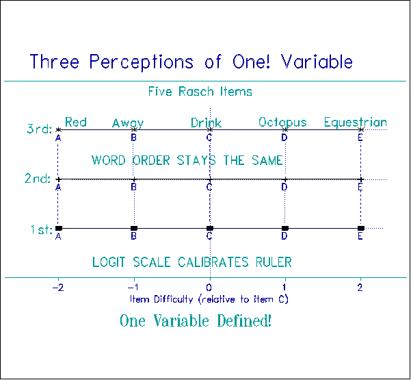
Figure 5 shows the relative locations of Rasch item calibrations for five words from Woodcock's ruler. It does not matter whether you are a 1st, 2nd or 3rd Grader, "red", "away", "drink", "octopus" and "equestrian" remain in the same order of experienced difficulty, at the same relative spacing. This ruler works the same way and defines the same variable for every child whatever their grade. It obeys the Magna Carta.
To obtain the construct stability manifest in Figure 5 we need the kind of item response curves which follow from the standard definition of fundamental measurement. Figure 6 shows that these Rasch curves do not cross. In fact, when we transform the vertical axis of these curves into log-odds instead of probabilities, the curves become parallel straight lines, thus demonstrating their conjoint additivity.
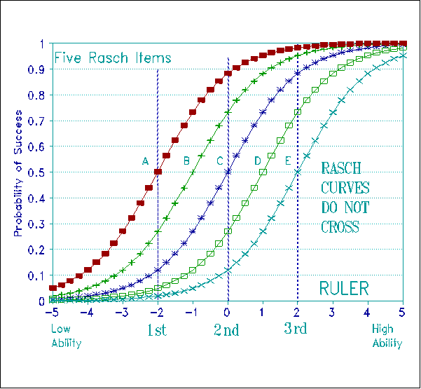
Figure 7, in contrast, shows five 3P Birnbaum curves for the same data. These five curves have different slopes and different asymptotes. There is no sign of conjoint additivity.
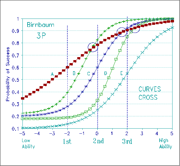
Figure 8 shows the construct destruction produced by the crossing curves of Figure 7. For a 1st Grader, "red" is said to be easier than "away" which is easier than "drink" which is easier than "octopus". But for a 3rd Grader the order of item difficulty is different. Now it is "away" rather than "red" that is easier. "Red" has become even harder than "drink"! And "octopus" is now almost as easy to recognize as "red", instead of being up near "equestrian". What is the criterion definition of this variable? What construct is defined? The definition is different at every ability level. There is no construct! No ruler! No Magna Carta!
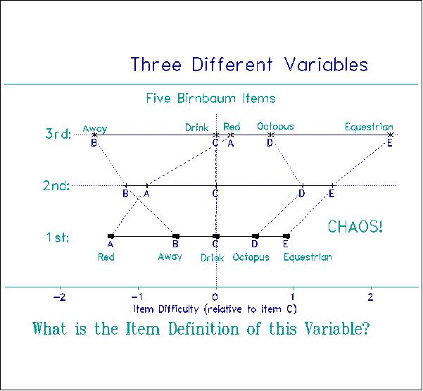
Much as we might be intrigued by the complexity of the Birnbaum 3P curves in Figure 7, we cannot use them to construct measures. To construct measures we require orderly, cooperating, non-crossing curves like the Rasch curves in Figure 6. This means that we must take the trouble to collect and refine data so that they serve this clearly defined purpose, so that they approximate a stochastic Guttman scale.
When we go to market, we eschew rotten fruit. When we make a salad, we demand fresh lettuce. We have a recipe for what we want. We select our ingredients to follow. It is the same with making measures. We must think when we select and prepare our data for analysis. It is foolish to swallow whatever comes. Our data must be directed to building a structure like the one in Figures 5 and 6 -- one ruler for everyone, everywhere, every time - so we can achieve a useful, stable construct definition like Woodcock's word-recognition ruler.
The lamentable history of the Birnbaum model is a cautionary tale of myopic promiscuity. Guessing is celebrated as an item asset. Discrimination is saluted as a useful scoring weight. Crossed item characteristic curves are swallowed without hesitation.
Models which build fundamental measurement are more choosy. They recognize guessing, not as an item asset but, as an unreliable person liability. They identify variation in discrimination as a symptom of item bias and multi-dimensionality (Masters, 1988). Instead of parameterizing discrimination and guessing and then forgetting them, models for fundamental measurement analyze the data for statistical symptoms of misfit including variations in discrimination and guessing, identify their item and person sources and weigh their impact on measurement quality.
In practice, guessing is easy to minimize. All one has to do is to test on target. Should a few lucky guesses crop up, it will not be items that produce them. The place to look for lucky guessing is among lucky guessers. The most efficient and fairest way to deal with lucky guessing, when it does occur, is to detect it, to measure the advantage it affords the lucky guesser, in case that matters, and, finally, to decide what is the most reasonable thing to do with the improbably successful responses that lucky guessing chanced on.
In the history of science there are vast differences between gerrymandering models to give best local descriptions of transient data and searching, instead, for better data that brings inferentially stable meaning to parameter estimates. It is the search for better data which begets discovery. The only way discovery can emerge is as an unexpected discrepancy from an otherwise stable frame of reference. When we study data misfit, we discover new things about what we are measuring and how people tell us about it. These discoveries strengthen and evolve our constructs as well as our ability to measure them.
The social history of stable units for fair trade makes clear that when units are unequal, when they vary from time to time and place to place, it is not only unfair, it is immoral. So too with the misuse of necessarily unequal and so unfair raw score units.
The purpose of measurement is inference. No measurement model which fails to meet the requirements for inference of probability, additivity, separability and divisibility can survive actual practice. Physics and Biology do not use and would never consider using models with intersecting trace lines. We measure to inform our plans for what to do next. If our measures are unreliable, if our units vary in unknown ways, our plans will go wrong and, eventually, our work will perish.
This simple point is sometimes belittled. It is not negotiable. It is vital and decisive! We will never build a useful, let along moral, social science until we stop deluding ourselves by analyzing local concrete ordinal raw scores as though they were general abstract linear measures.
Thurstone's "New" Measures
Thurstone outlined his necessities for a "new" measurement in the 1920's:
1. Measures must be linear, so that arithmetic can be done with them.
2. Item calibrations must not depend on whose responses they were estimated from - must be sample-free.
3. Person measures must not depend on which items they were estimated from - must be test-free.
4. Missing data must not matter.
5. The method must be easy to apply.
The mathematics needed to satisfy Thurstone's necessities and to make them practical were latent in Campbell's 1920 concatenation, Fisher's 1920 sufficiency and the divisibility of Levy and Kolmogorov and realized by Rasch's 1953 Poisson measurement model.
Rasch's "New" Models
The implications of Rasch's discovery have taken many years to reach practice (Wright 1968, 1977, 1984, Masters & Wright 1984). Even today there are social scientists who do not understand or benefit from what Campbell, Levy, Kolmogorov, Fisher and Rasch have proven (Wright 1992). Yet, despite this hesitation to use fundamental measurement models to transform raw scores into linear measures so that subsequent statistical analysis can become fruitful, there have been many successful applications (Wilson 1992, 1994, Fisher & Wright 1994, Engelhard & Wilson 1996, Wilson, Engelhard & Draney 1997).
Infinitely divisible (conjointly additive) models for the inverse probabilities of observed data enable:
1. The conjoint additivity which Norman Campbell (1920) and Luce and Tukey (1964) require for fundamental measurement (Brogden 1977, Perline, Wright & Wainer 1979, Wright 1985, 1988).
2. The exponential linearity which Ronald Fisher (1922) requires for estimation sufficiency (Andersen 1977, Wright 1989).
3. The parameter separability which Louis Thurstone (1925) and Rasch (1960) require for objectivity (Wright & Linacre 1989).
Measurement is an inference of values for infinitely divisible parameters which define the transition odds between observable increments of a theoretical variable.
No other formulation can construct results which a rational scientist, engineer, business man, tailor or cook would be willing to use as measures. Only data which can be understood and organized to fit this model can be useful for constructing measures. When data cannot be made to fit this model, the inevitable conclusion is that those data are inadequate and must be reconsidered (Wright 1977).
Rasch's models are applicable to every imaginable raw observation: dichotomies, rating scales, partial credits, binomial and Poisson counts (Andrich 1978, Masters & Wright 1984) in every reasonable observational situation including ratings faceted to: persons, items, judges and tasks (Linacre, 1989).
Computer programs which apply Rasch models have been in circulation for 30 years (Wright & Panchapakesan, 1969). Today, convenient, easy to use software for applying Rasch's "measuring functions" is readily available (Wright & Linacre 1997, Linacre & Wright 1997). Today it is easy for any social scientist to use computer programs like these to take the decisive step from unavoidably ambiguous concrete raw observations to well-defined abstract linear measures with realistic estimates of precision and explicit quality control. Today there is no methodological reason why social science cannot become as stable, as reproducible and as useful as physics.
Benjamin D. Wright
MESA Psychometric Laboratory
This paper was published as: Wright B.D. (1999) Fundamental measurement for psychology. In S.E. Embretson & S.L. Hershberger (Eds.), The new rules of measurement: What every educator and psychologist should know. Hillsdale, NJ: Lawrence Erlbaum Associates.
REFERENCES:
Andersen, E.B. (1977). Sufficient statistics and latent trait models. Psychometrika, (42), 69-81.
Andrich, D. (1978). A rating formulation for ordered response categories. Psychometrika, (43), 561-573.
Andrich, D. (1995). Models for measurement: precision and the non-dichotomization of graded responses. Psychometrika, (60), 7-26.
Andrich, D. (1996). Measurement criteria for choosing among models for graded responses. In A.von Eye and C.C.Clogg (Eds.), Analysis of Categorical Variables in Developmental Research. Orlando: Academic Press. 3-35.
Birnbaum A. (1968). Some latent trait models and their use in inferring an examinee's ability. In F.M.Lord and M.R.Novick, Statistical Theories of Mental Test Scores. Reading, Mass: Addison-Wesley.
Bookstein, A. (1992). Informetric Distributions, Parts I and II. Journal of the American Society for Information Science, 41(5):368-88.
Bookstein, A. (1996). Informetric Distributions. III. Ambiguity and Randomness. Journal of the American Society for Information Science, 48(1): 2-10.
Brogden, H.E. (1977). The Rasch model, the law of comparative judgement and additive conjoint measurement. Psychometrika, (42), 631-634.
Buchler, J. (1940). Philosophical Writings of Peirce. New York: Dover. 98-119.
Campbell, N.R. (1920). Physics: The elements. London: Cambridge University Press.
de Finetti, B. (1931). Funzione caratteristica di un fenomeno aleatorio. Atti dell R. Academia Nazionale dei Lincei, Serie 6. Memorie, Classe di Scienze Fisiche, Mathematice e Naturale, 4, 251-99. [added 2005, courtesy of George Karabatsos]
Eddington, A.S. (1946). Fundamental Theory. London: Cambridge University Press.
Embretson, S.E. (1998). Item response theory models and spurious interaction effects in multiple group comparisons. Applied Psychological Measurement.
Engelhard, G. (1991). Thorndike, Thurstone and Rasch: A comparison of their approaches to item-invariant measurement. Journal of Research and Development in Education, (24-2), 45-60.
Engelhard, G. (1994). Historical views of the concept of invariance in measurement theory. In Wilson, M. (Ed.), Objective Measurement: Theory into Practice Volume 2. Norwood, N.J.: Ablex, 73-99.
Engelhard, G. & Wilson, M. (Eds) (1996). Objective Measurement: Theory into Practice Volume 3. Norwood, N.J.: Ablex
Fechner, G.T. (1860). Elemente der psychophysik. Leipzig: Breitkopf & Hartel. [Translation: Adler, H.E. (1966). Elements of Psychophysics. New York: Holt, Rinehart & Winston.].
Feller, W. (1957). An Introduction to Probability Theory and Its Applications. New York: John Wiley & Sons.
Fischer, G. (1968). Psychologische Testtheorie. Bern: Huber.
Fisher, R.A. (1920). A mathematical examination of the methods of determining the accuracy of an observation by the mean error and by the mean square error. Monthly Notices of the Royal Astronomical Society, (53), 758-770.
Fisher, R.A. (1922). On the mathematical foundations of theoretical statistics. Philosophical Transactions of the Royal Society of London, (222), 309-368.
Fisher, W.P. & Wright, B.D. (1994). Applications of Probabilistic Conjoint Measurement. Special Issue. International Journal Educational Research, (21), 557-664.
Goldstein, H. (1980). Dimensionality, bias, independence and measurement scale problems in latent trait test score models. British Journal of Mathematical and Statistical Psychology, (33), 234-246.
Guttman, L. (1944). A basis for scaling quantitative data.
American Sociological Review,(9),139-150.
Guttman, L. (1950). The basis for scalogram analysis. In Stouffer et al. Measurement and Prediction, Volume 4. Princeton N.J.: Princeton University Press, 60-90.
Hambleton, R. & Martois, J. (1983). Evaluation of a test score prediction system. In R.Hambleton (Ed.), Applications of item response theory. Vancouver, BC: Educational Research Institute of British Columbia, 196-211.
Keats, J.A. (1967). Test theory. Annual Review of Psychology, (18), 217-238.
Kinston, W. (1985). Measurement and the structure of scientific analysis. Systems Research, 2, No, 2, 95-104.
Kolmogorov, A.N. (1950). Foundations of the Theory of Probability. New York: Chelsea Publishing.
Levy, P. (1937). Theorie de l'addition des variables aleatoires. Paris.
Linacre, J.M. (1989). Many-faceted Rasch Measurement. Chicago: MESA Press.
Linacre, J.M. & Wright, B.D. (1997). FACETS: Many-Faceted Rasch Analysis. Chicago: MESA Press.
Lord, F.M. (1968). An analysis of the Verbal Scholastic Aptitude Test Using Birnbaum's Three-Parameter Model. Educational and Psychological Measurement, 28, 989-1020.
Lord, F.M. (1975). Evaluation with artificial data of a procedure for estimating ability and item characteristic curve parameters. (Research Report RB-75-33). Princeton: ETS.
Luce, R.D. & Tukey, J.W. (1964). Simultaneous conjoint measurement. Journal of Mathematical Psychology,(1),1-27.
Masters, G.N. (1988). Item discrimination: When more is worse. Journal of Educational Measurement, (24), 15-29.
Masters, G.N. & Wright, B.D. (1984). The essential process in a family of measurement models. Psychometrika, (49), 529-544.
Perline, R., Wright, B.D. & Wainer, H. (1979). The Rasch model as additive conjoint measurement. Applied Psychological Measurement, (3), 237-255.
Rasch, G. (1960). Probabilistic models for some intelligence and attainment tests. [Danish Institute of Educational Research 1960, University of Chicago Press 1980, MESA Press 1993] Chicago: MESA Press.
Rasch, G. (1961). On general laws and meaning of measurement in psychology. Proceedings of the Fourth Berkeley Symposium on Mathematical Statistics and Probability, (4), 321-333. Berkeley: University of California Press.
Rasch, G. (1963). The Poisson process as a model for a diversity of behavioral phenomena. International Congress of Psychology. Washington, D.C.
Rasch, G. (1968). A mathematical theory of objectivity and its consequences for model construction. In Report from European Meeting on Statistics, Econometrics and Management Sciences. Amsterdam.
Rasch, G. (1969). Models for description of the time-space distribution of traffic accidents. Symposium on the Use of Statistical Methods in the Analysis of Road Accidents. Organization for Economic Cooperation and Development Report 9.
Rasch, G. (1977). On specific objectivity: An attempt at formalizing the request for generality and validity of scientific statements. Danish Yearbook of Philosophy, (14), 58-94. Copenhagen.
Samejima, F. (1997). Ability estimates that order individuals with consistent philosophies. Annual Meeting of the American Educational Research Association. Chicago: AERA.
Sears, S.D. (1997). A Monetary History of Iraq and Iran. Ph.D. Dissertation. Chicago: University of Chicago.
Sheriff, J.K. (1994). Charles Peirce's Guess at the Riddle. Bloomington: Indiana University Press. 41-47.
Smith, R.M. (1985). Validation of individual test response patterns. International Encyclopedia of Education, Oxford: Pergamon Press, 5410-5413.
Smith, R.M. (1986). Person fit in the Rasch Model. Educational and Psychological Measurement, (46), 359-372.
Smith, R.M. (1988). The distributional properties of Rasch standardized residuals. Educational and Psychological Measurement, (48), 657-667.
Smith, R.M. (1991). The distributional properties of Rasch item fit statistics. Educational and Psychological Measurement, (51), 541-565.
Smith, R.M. (1994). A comparison of the power of Rasch total and between item fit statistics to detect measurement disturbances. Educational and Psychological Measurement, (54), 42-55.
Smith, R.M. (1996). A comparison of methods for determining dimensionality. Structural Equation Modeling, 3(1), 25-40.
Stevens, S.S. (1939). On the problem of scales for the measurement of psychological magnitudes. Journal for the Unification of Science, (9), 94-99.
Stevens, S.S. (1946). On the theory of scales and measurement. Science, 103, 667-680.
Stigler, S.M. (1986). The History of Statistics. Cambridge: Harvard University Press.
Stocking, M.L. (1989). Empirical estimation errors in item response theory as a function of test properties. (Research Report RR-89-5). Princeton: ETS.
Swaminathan, H. (1983). Parameter estimation in item response models. In R.Hambleton (Ed.), Applications of item response theory. Vancouver, BC: Educational Research Institute of British Columbia, 24-44.
Thorndike, E.L. (1904). An introduction to the theory of mental and social measurements. New York: Teacher's College.
Thurstone, L.L. (1926). The scoring of individual performance. Journal of Educational Psychology, (17), 446-457.
Thurstone, L.L. (1928). Attitudes can be measured. American Journal of Sociology, (23), 529-554.
Thurstone, L.L. & Chave, E.J. (1929). The measurement of attitude. Chicago: University of Chicago Press.
Thurstone, L.L. (1931). Measurement of social attitudes. Journal of Abnormal and Social Psychology, (26), 249-269.
Wilson, M. (Ed) (1992). Objective Measurement: Theory into Practice Volume 1. Norwood, N.J.: Ablex.
Wilson, M. (Ed) (1994). Objective Measurement: Theory into Practice Volume 2. Norwood, N.J.: Ablex.
Wilson, M., Engelhard, G. & Draney, K. (Eds) (1997). Objective Measurement: Theory into Practice Volume 4. Norwood, N.J.: Ablex.
Woodcock, R.W. (1974). Woodcock Reading Mastery Tests. Circle Pines, Minn: American Guidance Service.
Wright, B.D. (1968). Sample-free test calibration and person measurement. Proceedings 1967 Invitational Conference on Testing Princeton: Educational Testing Service, 85-101.
Wright, B.D. (1977). Solving measurement problems with the Rasch model. Journal of Educational Measurement, (14), 97-116.
Wright, B.D. (1984). Despair and hope for educational measurement. Contemporary Education Review, (1), 281-288.
Wright, B.D. (1985). Additivity in psychological measurement. In Edw. Roskam (Ed.), Measurement and Personality Assessment. Amsterdam: North-Holland, 101-112.
Wright, B.D. (1988). Rasch model from Campbell concatenation for mental testing. In J.M.Linacre (Ed.) Rasch Measurement Transactions Part 1. Chicago: MESA Press, 1995, 16.
Wright, B.D. (1989). Rasch model from counting right answers. In J.M.Linacre (Ed.) Rasch Measurement Transactions Part 1. Chicago: MESA Press, 1995, 62.
Wright, B.D. (1992). IRT in the 1990's: Which models work best?. In J.M.Linacre (Ed.) Rasch Measurement Transactions Part 2. Chicago: MESA Press, 1996, 196-200.
Wright, B.D. (1994). Measuring and counting. In J.M.Linacre (Ed.) Rasch Measurement Transactions Part 2. Chicago: MESA Press, 1996, 371.
Wright, B.D. (1996). Comparing Rasch measurement and factor analysis. Structural Equation Modeling, 3(1), 3-24.
Wright, B.D. & Linacre, J.M. (1989). Observations are always ordinal: measures, however, must be interval. Archives of Physical Medicine and Rehabilitation, (70), 857-860.
Wright, B.D. & Linacre, J.M. (1997). BIGSTEPS: Rasch Computer Program for All Two Facet Problems. Chicago: MESA Press.
Wright, B.D. & Masters, G.N. (1982). Rating Scale Analysis: Rasch Measurement. Chicago: MESA Press.
Wright, B.D. & Panchapakesan, N. (1969). A procedure for sample-free item analysis. Educational and Psychological Measurement, (29), 23-48.
Wright, B.D. & Stone, M.H. (1979). Best Test Design: Rasch Measurement. Chicago: MESA Press.
Go to Top of Page
Go to Institute for Objective Measurement Page
| FORUM | Rasch Measurement Forum to discuss any Rasch-related topic |
| Coming Rasch-related Events | |
|---|---|
| May. 15 - June 12, 2026, Fri.-Fri. | On-line workshop: Rasch Measurement - Core Topics (E. Smith, Winsteps), www.statistics.com |
| June 19 - July 25, 2026, Fri.-Sat. | On-line workshop: Rasch Measurement - Further Topics (E. Smith, Winsteps), www.statistics.com |
| Aug. 31 - Sept 2 2026, Mon.-Wed. | In person: IMEKO TC1 Metrology Education and Training symposium, Klagenfurt, Austria www.photomet-edumet2026.com. Submissions by April 20 |
| Aug. 30 - Sept. 3, 2027, Mon.-Fri. | In Person: 2027 IMEKO World Congress (TC1, Tc7, TC13, TC18, TC26), Rimini, Italy imeko2027.org |
Our current URL is www.rasch.org
The URL of this page is www.rasch.org/memo64.htm